I remember looking at Gromov’s notes “Carnot-Carathéodory spaces seen from within” a long time ago and didn’t get anywhere. Recently I encountered it again through professor Guth. This time, with his effort in explaining, I did get some ideas. This thing is indeed pretty cool~ So I decided to write an elementary introduction about it here. We will construct a such metric in  .
.
In general, if we have a Riemannian manifold, the Riemannian distance between two given points  is defined as
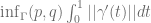
where  is the collection of all differentiable curves
  connecting the two points.
However, if we have a lower dimensional sub-bundle  of the tangent bundle (depending continuously on the base point). We may attempt to define the metric

where  is the collection of curves connecting with
  for all
  . (i.e. we are only allowed to go along directions in the sub-bundle.
Now if we attempt to do this in , the first thing we may try is let the sub-bundle be the say,  -plane at all points. It’s easy to realize that now we are ‘stuck’ in the same height: any two points with different
  coordinate will have no curve connecting them (hence the distance is infinite). The resulting metric space is real number many discrete copies of
  . Of course that’s no longer homeomorphic to .
Hence for the metric to be finite, we have to require accessibility of the sub-bundle: Any point is connected to any other point by a curve with derivatives in the .
For the metric to be equivalent to our original Riemannian metric (meaning generate the same topology), we need to be locally accessible: Any point less than  away from the original point
  can be connected to by a curve of length
  going along .
At the first glance the existence of a (non-trivial) such metric may not seem obvious. Let’s construct one on that generates the same topology:
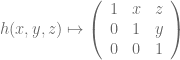
To start, we first identify our with the  real entry Heisenberg group
  (all upper triangular matrices with “1”s on the diagonal). i.e. we have homeomorphism
Let  be a left-invariant metric on
  .
.
In the Lie algebra  (tangent space of the identity element), the elements
 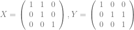 and
and  form a basis.
At each point, we take the two dimensional sub-bundle  of the tangent bundle generated by infinitesimal left translations by
  . Since the metric is left invariant, we are free to restrict the metric to i.e. we have
 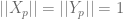 for each
  .
.
The interesting thing about is that all points are accessible from the origin via curves everywhere tangent to . In other words, any points can be obtained by left translating any other point by multiples of elements  and
and  .
.
The “unit grid” in under this sub-Riemannian metric looks something like:

Since we have
 ,
,
the original  -direction stay the same, i.e. a bunch of horizontal lines connecting the original
  planes orthogonally.
However, if we look at a translation by , we have
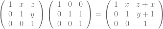
i.e. a unit length -vector not only add a  to the
  -direction but also adds a height to , hence the grid of unit vectors in the above three planes look like:

We can now try to see the rough shape of balls by only allowing ourselves to go along the unit grid formed by and lines constructed above. This corresponds to accessing all matrices with integer entry by words in and .
The first question to ask is perhaps how to go from  to
to  . –since going along the axis is disabled. Observe that going through the following loop works:

We conclude that  in fact up to a constant going along such loop gives the actual distance.
At this point one might feel that going along axis in the C-C metric is always takes longer than the ordinary distance. Giving it a bit more thought, we will find this is NOT the case: Imagine what happens if we want to go from to  ?
?
One way to do this is to go along for 100 steps, then along for 100 steps (at this point each step in will raise  in -coordinate, then
  . This gives
  .
.
To illustrate, let’s first see the loop from to  :
:

The loop has length  . (A lot shorter compare to length
  for going unit in -direction)
i.e. for large  , it’s much more efficient to travel in the C-C metric.
In fact, we can see the ball of radius  is roughly an rectangle with dimension
  (meaning bounded from both inside and outside with a constant factor). Hence the volume of balls grow like
  .
.

Balls are very “flat” when they are small and very “long” when they are large.
40.342975
-74.651315


Finally I can read your blog….
So happy about it.
LikeLike
Thank you! (although I can’t recall who you are…>.<)
LikeLike
ABC on your xiaonei….
LikeLike
Hello, Conan.
Why is this Lie algebra generated by matrices with 1 on diagonal? H_3 is a subgroup of SL(3), so it’s Lie algebra elements must have zero traces, am I right?
And how to build continous curve using transformation of type 2 (multiplication by Y)?
Sorry for my English and sorry if questions are stupid.
Thank you!
Kostya
LikeLike
Hi Kostya,
Thanks a lot for the comment~
When I say ‘Lie algebra’, in fact I meant since the space is itself linear, I’m considering the tangent space as embedded subspace at identity. Yes you are right that I should write all the element as the current ones minus identity and when I need to multiply them, add identity again…but hopefully the idea is pretty clear, right?
Going from discrete to continuous is merely going infinitesimally to tangent vectors instead of multiply by the integer matrix Y each time, right? (i.e. Y in the Lie algebra determines a left-invariant vector field, hence one can find curves tangent to Y in the Lie group)
Please note that I know very little about Lie groups, hence whatever I say about them perhaps contain many wrong terminolo >.<
Feel free to point out any mistakes or suggest better ways to state things.
Best,
Conan
LikeLike
Thank you for your answer!
I’m myself very bad with Lie groups, sorry, it was rather obvious. But it is not about substracting identity of course, it’s about exponential map, in our case exp(X) = E + X (this is just to clear it for myself, I’m sure that this is what you originally said, and I just had not enough expirience to understand).
All right, now it is clear, thank you very much for your post!
Best,
Kostya
LikeLike
[…] The Carnot-Carathéodory metric […]
LikeLike