This article was written as a homework of professor Wilkinson’s dynamical systems course. Since the content is expository and detailed presentation of the theorem is missing from many books, I decided to post it here. I have mostly followed a set of notes by John Franks, with additional discussions on the intuition and ideas behind the statement and the proof.

1.Introduction

So far we have discussed various different kinds of dynamical systems ranging from topological, smooth to hyperbolic and partially hyperbolic. One might wonder if there is a united theme to the subject as a whole. Indeed, as in many other subjects, there is a so-called fundamental theorem of dynamical systems. This theorem is first stated and proved by Conley in where he studies attractor and repellers. The theorem, loosely speaking, gives a universal decomposition of any systems on compact metric spaces into invariant compact sets wandering orbits that travels between such sets.

To state this more precisely we make an analogy with Morse theory: When looking at the gradient flow on a compact embedded manifold, we ‘decompose’ the manifold into critical points and orbits that originates and ends at critical points. In a similar spirit, given any homeomorphisms on a compact metric space, we may look at it’s ‘indecomposible’ compact invariant sets and how they are ‘connected’ by wandering orbits, we then ‘place’ those compact sets on different ‘heights’ and have all other point going between the minimal sets they originates and ends at. The theorem guarantees that we can ‘place’ the space in a way that all wandering orbits are going ‘down’ at all times.

In light of the theorem, we have descried the global structure of the system except for what happens on the ‘indecomposible’ sets. i.e. The problem of understanding general topological systems on compact manifolds is reduced to understanding ‘transitive’ homeomorphisms on compact sets. The latter, unfortunately, could still be quite complicated as we have seen in the Horseshoe example.

The theorem is proposed to be the Fundemental theorem of dynamical systems because of its nature in giving concise description of all possible behaviors of a system in the given setting. In some sense, dynamics is the study of limiting behrviors of all points under interation, the theorem breaks the system down into a recurrent part and a wandering part where the behavior of the wandering part is gradient-like. Since we have developped sets of different tools for studying systems that exhibits a lot of recurrence as well as for studying gradient-like systems, this allows us to connect combine the tool sets and treat any systems in the setting.

2.Background

In this section, we define -chains, chain recurrent sets and chain transitive components for a homeomorphism on a compact metric space. Those concepts will come up in the statement of the fundamental theorem. In fact, those are going to be the ‘minimal compact sets’ we decompose our metric space into.

Given compact metric space and homeomorphism ,
Definition: Given two points , an -chain from to is a sequence , where and for all , .

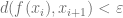
i.e. we take a point and start applying to it, but at each iterate, we are allowed to perturb the resulting point by . Such ‘pseudo-orbits’ are in general much easier to obtain than true orbits.

More generally, -chains can be taken infinite. i.e. if we have a (possibly infinite) subinterval , an -chain indexed by is a set of points s.t. whenever are both in .

Definition: is chain recurrent if for all , there exists an -chain from to itself. The set of all chain recurrent points in is called the \textbf{chain recurrent set}, denoted by .

Note that non-wandering points are necessarily chain recurrent: If 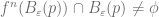is non-wandering, we may take the neighborhood to be the -ball around , since is non-wandering, we have some where , we pick in the intersection and define -chain .

At this point, it’s perhaps worthwhile to mention our completed ordering of different notions of recurrence:

Each of the above inclusion can be made strict (see Exercises). Chain recurrence is perhaps the weakest notion I’ve seen for a point to be, in any sense, recurrent. A Friendly challenge to the reader: think of a case where you feel confortable calling a point ‘recurrent’ while it’s not in the chain recurrent set of the system.

We now define equivlence relation on as follows:

For in , iff for all , there are -chains from to and from to . is reflexive since all points in are chain recurrent; symmetric by definition and transitive by the obvious composition of -chains.

Definition: The equivalence classes in for are called chain transitive components.

It’s easy to check that chain transitive components are compact and -invariant. Those are components that’s transitive in a very weak sense. i.e. any two points are connected by a ‘pseudo-orbit’, or equivalently, there is a dense (infinite) pseudo-orbit. (see exercises)

As mentioned above, throughout the rest of the chapter, we will consider chain transitive components as ‘indecomposible parts’ of our system. Those are the parts for which all points are ‘recurrently’ and each component is ‘transitive’, both in a very weak sense. We further specify how does the points that are not in the chain-recurrent set iterates between those components.

3.Statement of the theorem

Given compact metric space and homeomorphism ,

Definition: is a complete Lyapunov function for if:

Hence this is a function that stays constant only on the chain transitive components and strictly decreases along any orbit not in . We also require the image of to be compact and nowhere dense which cooresponds to the ‘critical values’ of a gradient function being compact nowhere dense as a result of Sard’s theorem.

Fundemental theorem of dynamical systems:

Complete Lyapunov function exists for any homeomorphisms on compact metric spaces.

As a historical remark, the theorem first appeared in Charles Conley’s CBMS monograph Isolated Invariant Sets and the Morse Index in 1978 [C]. In the book he developed the theory of attractor-repeller pairs in relation to Morse decomposition and index theory. The above theorem was one of the major results. Although Conley was originally more focused on the setting where instead of a homeomorphism, we have a continuous flow on the manifold (which makes it even more similar to the gradient flow), but this discrete formulation became more popular as the theory develops. The theorem is later proposed by D. Norton as the fundamental theorem of dynamical in 1995.

The proof is going to be a specific construction: First, we define a family of partitions of the chain recurrent set, each divides the set into two pieces (i.e. a attractor-repeller pair intersected with ). Then we prove the family is countable and points in the same chain transitive component are not separated by any partition in the family. Furthermore, each chain-transitive component is uniquely defined by specifying which set does it belong to in each partition. i.e. the smallest common refinement for the family exactly partitions into chain-transitive components. (section 4)

Next, for each attractor-repeller pair, we prove the existence of a function that takes value on the attractor and on the repeller and strictly decreases along orbits of points that’s not in . We should also mention the fact that all points that are contained in one of the sets in each pair must be in chain recurrent. (section 5)

The complete Lyapunov function is then constructed by taking an appropriate infinite sum of such functions. This way we get a function that separates all chain transitive components, stays constant on each component and strictly decreases along all orbits which are not in . The image of the chain recurrent set will be contained in the middle-third Cantor set. (section 6)

(see part 2 for sections 4-6)