In the past few years, there are 137 papers with the term ‘sumset’ in its title; and 50 more with ‘sum-set’. Ok the above statement was stolen from a talk I happen to be sitting in, by Noga Alon.
As usual, in the middle of the talk I got carried away by some ‘trivial facts’ he wrote down which are only slightly related to the main content. So I thought about that for during the rest of the talk (and also a little bit afterwards).
This time the curious point pops up when he was motivating why people should be studying chromatic number of random Cayley graphs by its application to sumsets.
Definition: In a vector space 


It was mentioned that given a large 

This fact is first published by Ben Green who also raised the natural question:
Question: What’s the lower bound 


Let’s first see why all sets of large cardinality must be sumsets: Well as we all know 

The way I think of sumsets is that they are projections of product sets in the angle 

Hence our goal is to make up a set 


Note that since 

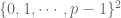
So we just showed all sets with one missing element is a sumset~ Now let’s move to sets of size 
In contrast to the above argument which actually works in the continuous setting and shows the Lie group 
Note first that the property of being a sumset is invariant under scaling and translating by an integer. Indeed,

and of course 
Now no matter which two points 

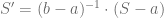


Hence ![S = [(b-a) \cdot I + a/2] + [(b-a) \cdot I + a/2]](https://s0.wp.com/latex.php?latex=S+%3D+%5B%28b-a%29+%5Ccdot+I+%2B+a%2F2%5D+%2B+%5B%28b-a%29+%5Ccdot+I+%2B+a%2F2%5D+&bg=ffffff&fg=5e5e5e&s=0&c=20201002)
After playing around with the torus for a little bit, I believe in the continue case we can still write 


(By the way, this is about as far as I got daydreaming during the lecture, the rest came from the sources I looked up afterwards.)
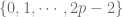
Unfortunately since the scaling and translating gived only two degrees of freedom, the above argument fails when considering sets missing three points. (Playing with torus as I first tried, however, might still work)
Back to our question, so now we know at least 


So this is quite curious, what do you think? Is 

As one might have expected,
Theorem: (Green) 
It’s also not as large as a fixed percentage:
Theorem: (Gowers-Green)
So it’s something ‘in-between’. Interesting…So what is this number? This is an open question in general, by applying methods of Cayley graphs and their spectrums, the speaker (of the talk) was able to improve the above bounds (in this other paper):
Theorem: (Alon)

However one should expect that
Conjecture: (Green) 
Having knowing absolutely nothing about the subject (or combinatorics in general), my first reaction about this is that perhaps, if we look at 


I think this set looks (by the same philosophy as when we play around with the two intervals on the tori case) fairly hard to express as a sum. i.e. when we are exactly in 
Anyways, that last remark might be completely nonsense~ The conjecture is interesting, tho.
 , we define the k-codimensional width (or simply k-width) to be the smallest possible number
  where there exists a k-dimensional affine subspace
  s.t. all points of
  .
.
 is the length of the orthogonal segment from
  .
. . However it is not the case since for example the equilateral triangle of side length
  in
in  has diameter
  . In fact, by a theorem of
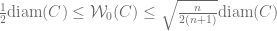
 where there is an orthogonal projection of
  dimensional subspace
  has pre-image with diameter
  .
.
 .
. , unlike
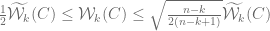
 iff
iff  is the smallest number
  where any point
  has pre-image with diameter
  .
.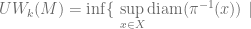

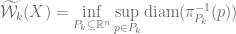
 dimensional if any finite cover of
  sets in the cover and
  since the pair
  is clearly among the pairs we are minimizing over.
![M=[0,1]^n](https://s0.wp.com/latex.php?latex=M%3D%5B0%2C1%5D%5En&bg=ffffff&fg=5e5e5e&s=0&c=20201002) be the solid n-dimensional cube, then for any topological space
be the solid n-dimensional cube, then for any topological space  and any continuous map
  , we have image of at least one pair of opposite
  -faces intersect.
![M = [0, L_1] \times [0, L_2] \times \cdots \times [0, L_n]](https://s0.wp.com/latex.php?latex=M+%3D+%5B0%2C+L_1%5D+%5Ctimes+%5B0%2C+L_2%5D+%5Ctimes+%5Ccdots+%5Ctimes+%5B0%2C+L_n%5D&bg=ffffff&fg=5e5e5e&s=0&c=20201002) ,
,  , we have
  ; furthermore,
  for all
  ,
,  being the product of the first
  coordinates. Now
  ).
). then the notion is the same as the minimax length of fibres. In particular as proved in the post the minimax length of the unit disc to
  is 2.
is 2. , i.e. the optimum is obtained by contracting the disc onto a triod.
 neighborhood of a tree will have
  about
about  .
. if for every
  , saturating the set
  . In deed this is the case:
 iff the
  has all
  (Hausdorff dimension), let
  be the Garssmann manifold consisting of all
  ,
,  for almost all
 ,
,  has positive
  .
. of
of  . For any point
  , there exists a small neighborhood in which the foliation is diffeomorphic to the subspace foliation of the Euclidean space. i.e. there exists
  from a neighborhood
  of
of  where the leaves of
  ,
,  .
. to be half of the origional
  is the same as
  saturated by parallel
  is the same as dimension of
  , if the inequality is strict, then all projections of