Recently I came across a paper by John Pardon – a senior undergrad here at Princeton; in which he answered a question by Gromov regarding “knot distortion”. I found the paper being pretty cool, hence I wish to highlight the ideas here and perhaps give a more pictorial exposition.
This version is a bit different from one in the paper and is the improved version he had after taking some suggestions from professor Gabai. (and the bound was improved to a linear one)
Definition: Given a rectifiable Jordan curve  , the distortion of
  is defined as
 .
.
i.e. the maximum ratio between distance on the curve and the distance after embedding. Indeed one should think of this as measuring how much the embedding ‘distort’ the metric.
Given knot  , define the distortion of to be the infimum of distortion over all possible embedding of :

It was (somewhat surprisingly) an open problem whether there exists knots with arbitrarily large distortion.
Question: (Gromov ’83) Does there exist a sequence of knots  where
where  ?
?
Now comes the main result in the paper: (In fact he proved a more general version with knots on genus  surfaces, for simplicity of notation I would focus only on torus knots)
Theorem: (Pardon) For the torus knot  , we have

.
To prove this, let’s make a few observations first:
First, fix a standard embedding of  in
in  (say the surface obtained by rotating the unit circle centered at
  around the
  -axis:

and we shall consider the knot that evenly warps around the standard torus the ‘standard knot’ (here’s what the ‘standard  knot looks like:

By definition, an ’embedding of the knot’, is a homeomorphism  that carries the standard to the ‘distorted knot’. Hence the knot will lie on the image of the torus (perhaps badly distorted):


For the rest of the post, we denote  by and
  by
by  , w.l.o.g. we also suppose
  .
.
Definition: A set  is inessential if it contains no homotopically non-trivial loop on .
Some important facts:
Fact 1: Any homotopically non-trivial loop on that bounds a disc disjoint from intersects at least  times. (hence the same holds for the embedded copy
  ).
).
As an example, here’s what happens to the two generators of  (they have at least and
  intersections with respectively:

From there we should expect all loops to have at least that many intersections.
Fact 2: For any curve and any cylinder set ![C = U \times [z_1, z_2]](https://s0.wp.com/latex.php?latex=C+%3D+U+%5Ctimes+%5Bz_1%2C+z_2%5D&bg=ffffff&fg=5e5e5e&s=0&c=20201002) where
where  is in the
  -plane, let
  we have:
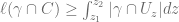
i.e. The length of a curve in the cylinder set is at least the integral over -axis of the intersection number with the level-discs.
This is merely saying the curve is longer than its ‘vertical variation’:

Similarly, by considering variation in the radial direction, we also have

Proof of the theorem
Now suppose  , we find an embedding with
  .
.
For any point  , let
, let
 is inessential
i.e. one should consider  as the smallest radius around
  so that the whole ‘genus’ of lies in
  .
.
It’s easy to see that  is a positive Lipschitz function on that blows up at infinity. Hence the minimum value is achieved. Pick
  where is minimized.
Rescale the whole so that  is at the origin and
  .
.
Since  (and note distortion is invariant under scaling), we have

Hence by fact 2, 
i.e. There exists ![R \in [1, \frac{11}{10}]](https://s0.wp.com/latex.php?latex=R+%5Cin+%5B1%2C+%5Cfrac%7B11%7D%7B10%7D%5D&bg=ffffff&fg=5e5e5e&s=0&c=20201002) where the intersection number is less or equal to the average. i.e.
where the intersection number is less or equal to the average. i.e. 
We will drive a contradiction by showing there exists with  .
.
Let ![C_z = B(\bar{0},R) \cap \{z \in [-\frac{1}{10}, \frac{1}{10}] \}](https://s0.wp.com/latex.php?latex=C_z+%3D+B%28%5Cbar%7B0%7D%2CR%29+%5Ccap+%5C%7Bz+%5Cin+%5B-%5Cfrac%7B1%7D%7B10%7D%2C+%5Cfrac%7B1%7D%7B10%7D%5D+%5C%7D&bg=ffffff&fg=5e5e5e&s=0&c=20201002) , since
, since

By fact 2, there exists ![z_0 \in [-\frac{1}{10}, \frac{1}{10}]](https://s0.wp.com/latex.php?latex=z_0+%5Cin+%5B-%5Cfrac%7B1%7D%7B10%7D%2C+%5Cfrac%7B1%7D%7B10%7D%5D&bg=ffffff&fg=5e5e5e&s=0&c=20201002) s.t.
s.t.  . As in the pervious post, we call
  a ‘neck’ and the solid upper and lower ‘hemispheres’ separated by the neck are
  .
.

Claim: One of  is inessential.
Proof: We now construct a ‘cutting homotopy’  of the sphere
  :
:

i.e. for each  is a sphere; at
  it splits to two spheres. (the space between the upper and lower halves is only there for easier visualization)
Note that during the whole process the intersection number  is monotonically increasing. Since
 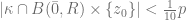 , it increases no more than
  .
.
Observe that under such ‘cutting homotopy’,  is inessential then
  is also inessential. (to ‘cut through the genus’ requires at least many intersections at some stage of the cutting process, but we have less than
  many interesections)
Since  is disconnected, the ‘genus’ can only lie in one of the spheres, we have one of is inessential. Establishes the claim.
We now apply the process again to the ‘essential’ hemisphere to find a neck in the  direction, i.e.cutting the hemisphere in half in
  direction, then the
  -direction:

The last cutting homotopy has at most  many intersections, hence has inessential complement.
Hence at the end we have an approximate  ball with each side having length at most
  , this shape certainly lies inside some ball of radius
  .
.

Let the center of the -ball be . Since the complement of the ball intersects in an inessential set, we have  is inessential. i.e.

Contradiction.
42.054805
-87.676354


 , embed a thinner torus
  as shown:
 into
into  so that

![C \times [0,1]](https://s0.wp.com/latex.php?latex=C+%5Ctimes+%5B0%2C1%5D&bg=ffffff&fg=5e5e5e&s=0&c=20201002) where
where  is the standard middle-third Cantor set. Bend them into Rainbow-shape with the open ends facing each other:
 ‘brush’ with ink only on the points of the Cantor set, and use the brush to draw two semicircles)
 brush and connect the top pair of ends so that they link with each other, and then a width
  brush for the highest remaining pair, etc. Take the union of all those connecting sets, union a line segment joining the bottom-most pair of points, we get the Whitehead continuum:
 in the three-sphere
  , equipped with the
  is null-homotopic in
  .
. is contractible to a loop in


 at some finite time)
 . Now by performing the operation above, we can homotope all parts of the loop that goes through the
  -gaps, by having the segments crossing themselves once. Now we pass to the
  -gaps, etc. until the loop lie completely outside the thickened disc which the continua lies in. Once it’s outside the disc, the loop can be contracted.
 form a thickened Whitehead link:

 handlebody. The resulting manifold (after taking the complement of the intersection) is a homotopy genus
  handlebody. (As in the whitehead case,


 i.e. all adjecent faces are orthogonal in the hyperbolic space. But this is achieved if we inscribe the regular octahedron into the Klein model (also called projective model of hyperbolic 3-space.