In the book “Elementary number theory, group theory and Ramanujan graphs“, Sarnak et. al. gave an elementary construction of expander graphs. We decided to go through the construction in the small seminar and I am recently assigned to give a talk about the girth estimate of such graphs.
Given graph (finite and undirected)  , we will denote the set of vertices by
  and the set of edges
  . The graph is assumed to be equipped with the standard metric where each edge has length
  .
.
The Cheeger constant (or isoperimetric constant of a graph, see this pervious post) is defined to be:
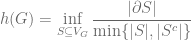
Here the notation  denote the set of edges connecting an element in
  to an element outside of .
Note that this is indeed like our usual isoperimetric inequalities since it’s the smallest possible ratio between size of the boundary and size of the set it encloses. In other words, this calculates the most efficient way of using small boundary to enclose areas as large as possible.
It’s of interest to find graphs with large Cheeger constant (since small Cheeger constant is easy to make: take two large graphs and connect them with a single edge).
It’s also intuitive that as the number of edges going out from each vertice become large, the Cheeger constant will become large. Hence it make sense to restrict ourselves to graphs where there are exactly  edges shearing each vertex, those are called -regular graphs.
If you play around a little bit, you will find that it’s not easy to build large k-regular graphs with Cheeger constant larger than a fixed number, say,  .
.
Definition: A sequence of k-regular graphs  where
where  is said to be an expander family if there exists constant
  where
where  for all
  .
.
By random methods due to Erdos, we can prove that expander families exist. However an explicit construction is much harder.
Definition: The girth of is the smallest non-trivial cycle contained in . (Doesn’t this smell like systole? :-P)
In the case of trees, since it does not contain any non-trivial cycle, define the girth to be infinity.
The book constructs for us, given pair  of primes where
  is large (but fixed) and
  , a graph
  -regular graph
 with
with
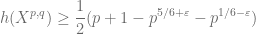
where  .
.
Note that the bound is strictly positive and independent of  . Giving us for each ,
  as q runs through primes larger than
  is a -regular expander family.
In fact, this constructs for us an infinite family of expander families: a  -regular one for each prime and the uniform bound on Cheeger constant gets larger as becomes larger.
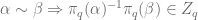
One of the crucial step in proving this is to bound the girth of the graph , i.e. they showed that  and if the quadratic reciprocity
  then
then 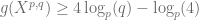 . This is what I am going to do in this post.
Let  be the set of quaternions with
  coefficient, i.e.

Fix odd prime , let


where the norm  on
on  is the usual
  .
.
 consists of points with only odd first coordinate or points lying on spheres of radius
  and having only even first coordinate. One can easily check is closed under multiplication.
Define equivalence relation  on by
on by
 if there exists
  s.t.
s.t.  .
.
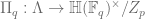
Let  , let
, let  be the quotient map.
Since we know  ,
,  carries an induced multiplication with unit.
In elementary number theory, we know that the equation  has exactly
  integer solutions. Hence the sphere of radius in contain points.
In each  -tuple
  exactly one is of a different parity from the rest, depending on whether
  or
or  . Restricting to solutions where the first coordinate is non-negative, having different parity from the rest (in case the first coordinate is
  , we pick one of the two solutions
  to be canonical), this way we obtain exactly
  solutions.
Let  be this set of points on the sphere. Note that the
  s represent the solutions where the first coordinate is exactly .
Check that  generates .
We have  and
and  . By definition
  and
and  is injective on . Let
  .
.
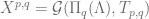
Consider the Cayley graph  , this is a -regular graph. Since
  generares , is connected.
Claim: is a tree.
Suppose not, let  a non-trivial cycle.
  . Since
  is a Cayley graph, we may assume
  .
.
Hence  , for some
  .
.
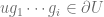
Since  for all
  , the word
  cannot contain either
  or
or  , hence cannot be further reduced.
 in means for some
  we have
 .
.
Since every word in with norm  must have a unique factorization
  where
where  is a reduces word of length
  in and
  .
.
Contradiction. Establishes the claim.
Now we reduce the group  mod :
mod :

One can check that  .
.
Let  ,
,  is a central subgroup.
For  ,
,  . Which means we have well defined homomorphism
 .
.
Let  , if
, if  we have
  is injective on and hence $latex
  .
.
Now we are ready to define our expanding family:
 .
.
Since generates ,  generates
  . Hence is -regular and connected.
Theorem 1:
Let  be a cycle in , there is
  such that
  for
for  .
.
Let  ,
,  . Note that from the above arguement we know
  is a reduced word, hence
  . In particular, this implies
  cannot all be .
Also, since is reduced,  .
.
By Lemma, since  ,
,  hence divide , we conclude

We deduce  hence
hence  for all cycle. i.e.
  .
.
Theorem 2: If does not divide and is not a square mod (i.e. ), then .
For any cycle of length as above, we have  , i.e.
  .
.
Since  , we have
  is even. Let
  .
.
Note that  , we also have
Hence  .
.
Since  ,
,  .
.
If  we will have
  . Then
  .
.
But we know that , one of  must be divisible by
  , hence .
Conclude  ,
,  , hence
  . Contradiction.
40.343599
-74.651774


 , for any
  , there exists
  such that any normed vector space of dimension
  into the Hilbert space.
 ) for any given k, *any* norm on a vector space of sufficiently high dimension will have a
  , does there exist a
  has a subset
  that embeds into the Hilbert space with distorsion
  such that for any
  , every compact metric space with dimension
  that admits an embedding into Hilbert space with distorsion
  .
. of course blows up to infinity whenever
  or
or  . (whenever we need a huge dimensional space with fixed ‘flatness’ or a fixed dimension but ‘super-flat’ subspace). That is, when we are looking for subspaces inside a random space with fixed (large) dimension
  necessarily forces
  and
and .
. is close to
  ! In fact, when we are allowing relatively large distorsion (compare to constant
  and a family of metric spaces
  such that for any small
  with dimension
  embeds into Hilbert space with distorsion
  .
. , there is no
  , in the paper they also produced spaces
  are of Hausdorff dimension 0!
 is a metric with the additional property that for any three points
  , we have the so-called strong triangle inequality, i.e.
 , with the dictionary metric (two points are distance
  apart where
  . It’s not hard to see in fact all such space embeds isometrically in
  by a Lipschitz map.
 Heegaard splittings of a
  is a decomposition of the manifold as a union of two handlebodies intersecting at the boundary surface. The genus of the Heegaard splitting is the genus of the boundary surface.
 is a surgery on
 ![F_g \times [0,1]](https://s0.wp.com/latex.php?latex=F_g+%5Ctimes+%5B0%2C1%5D&bg=ffffff&fg=5e5e5e&s=0&c=20201002) with the two ends identified by some diffeomorphism
with the two ends identified by some diffeomorphism  ,
,  ):
):
 be the
  (i.e. glue together $k$ copies of
  all via the map
 be the manifold obtained by cut open
  at the ends:
 we can choose a large enough
  , let
, let  be the union of handlebody
  together with the first
  be
be  with the last
  are genus
 and
and  cannot be made equivalent by less than
  . That would mean that we can sweep through the manifold by a surface of genus (at most)
  .
. everywhere, for any given genus
  , one can isotope the sweep-out so that each surface in the sweep-out having area
  .
. sweep-out harmonic for each
  in half. Furthermore, the time 1 half-volume-surface is roughly same as the time 0 surface with two sides switched.
  surface, all having volume less than some constant independent of
  , there is
  and area
  inside the middle fibred manifold with boundary
  bounds a
  where
where .
. in half and flips the two sides of the surface as time goes from
  for all
  and intersect them with the left-most
  (call it
  ), at some
  and
and  .
. and
and  has genus
  ! (say it's
 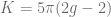 , there is
  .” or equivalently, given
  bounded open, we always have
 , we have
 is the volume of the unit n-ball. Note that the inequality is sharp for balls in
  be its Cayley graph, equipped with the word metric
  .
. be the cardinality of the ball of radius
  around the identity.
 , we define
  i.e. points that’s not in
  but there is an edge in the Cayley graph connecting it to some point in
  , then for any set
  ,
, .
. , so we have
  .
. , we look at how many elements of
  . (Here the idea being the size of the boundary can be lower bounded in terms of the length of the translation vector and the volume shifted outside the set. Hence we are interested in finding an element that’s not too far away from the identity but shifts a large volume of
  as
as  is:
is: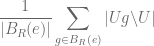
 , count how many
  outside
  .
. .
. , hence
  .
. 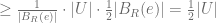
 (at least as large as average).
 .
. , since
  , there must be some
  s.t.
s.t.  and
and  .
.  ,
,  .
. i.e. a union of
  .
.

 , we have
  .
.  , hence we have
 , then trancing through the argument we get bound
 . But to get that one needs to use more information of the expander than merely the volume of balls.
 then for any open set
  .
. is above average.
 ![\gamma: [0, ||g||]](https://s0.wp.com/latex.php?latex=%5Cgamma%3A+%5B0%2C+%7C%7Cg%7C%7C%5D&bg=ffffff&fg=5e5e5e&s=0&c=20201002) be a unit speed geodesic connecting
be a unit speed geodesic connecting  to
to ![\gamma([0, ||g||])](https://s0.wp.com/latex.php?latex=%5Cgamma%28%5B0%2C+%7C%7Cg%7C%7C%5D%29&bg=ffffff&fg=5e5e5e&s=0&c=20201002) , this must contain all of
, this must contain all of  since for any
  the segment
 ![\gamma([0,||g||]) \cdot u](https://s0.wp.com/latex.php?latex=%5Cgamma%28%5B0%2C%7C%7Cg%7C%7C%5D%29+%5Ccdot+u&bg=ffffff&fg=5e5e5e&s=0&c=20201002) must cross the boundary of
must cross the boundary of ![c \in [0,||g||]](https://s0.wp.com/latex.php?latex=c+%5Cin+%5B0%2C%7C%7Cg%7C%7C%5D&bg=ffffff&fg=5e5e5e&s=0&c=20201002) where
where  , hence
 .
.

 .
. 