Hi guys~ The school year here at Princeton is finally (gradually) starting. So I’m back to this blog :-P
In this past week before anything has started, Assaf Naor came here and gave a couple rather interesting talks, which I decided to make a note about. For the complete content of the talk please refer to this paper by Naor and Mendel. As usual, I make no attempt on covering what was written on the paper nor what was presented in the talk, just some random pieces and bits which I found interesting.
A long time ago, Grothendieck conjectured what is now known as Dvoretzky’s theorem:
Theorem: For any 


i.e. this says in the case where 


Well, that’s pretty cool, but linear. As we all know, general metric spaces can be much worse than normed vector spaces. So here comes a nonlinear version of the above, posted by Terrence Tao:
Nonlinear Dvoretzky problem: Given 


Indeed, we should expect this to be a lot more general and much harder than the linear version, since we know literally nothing about the space except for having large Hausdorff dimension and as we know metric spaces can be pretty bizarre. That why we should find the this new result of theirs amazing:
Theorem 1 (Mendel-Naor): There is a constant 


Note that, in the original linear problem, 


We can see that this nonlinear theorem is great when we need large dimensional subspaces (when 

In the original statement of the problem this gives not only that a large 
Theorem 2 (Mendel-Naor): There exists constant 


This construction makes use of our all-time favorite: expander graphs! (see pervious post for definitions)
So what if 


In his words, the proof of theorem 1 (i.e. the paper) takes five hours to explain, hence I will not do that. But among many neat things appeared in the proof, instead of embedding into the Hilbert space directly they embedded it into an ultrametric space with distorsion
Definition: An ultrametric on space 


If one pause and think a bit, this is a quite weird condition: for example, all triangles in an ultrametric space are isosceles with the two same length edge both longer than the third edge; every point is the center of the ball, etc.
Exercise: Come up with an example of an ultrametric that’s not the discrete metric, on an infinite space.
Not so easy, hum? My guess: the first one you came up with is the space of all words in 2-element alphabet 


In fact in some sense all ultrametrics look like that. (i.e. they are represented by an infinite tree with weights assigned to vertices, in the above case a 2-regular tree with equal weights on same level) Topologically our 
I just want to say that this operation of first construct an ultrametric space according to our given metric space, embed, and then embed the ultrametric metric space into the Hilbert space somehow reminds me of when we want to construct a measure satisfying a certain property, we first construct it on a Cantor set, then divide up the space and use the values on parts of the Cantor set for parts of the space…On this vein the whole problem gets translated to producing a tree that gives the ultrametric and work with the tree (by no means simple, though).
Finally, let’s see a cute statement which can be proved by applying this result:
Urbanski’s conjecture: Any compact metric space of Hausdorff dimension > 
(note strictly larger is important for our theorem to apply…since we need to subtract an
Question: Does any compact metric space with positive Hausdorff
 .
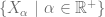
. is defined as
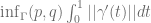
 is the collection of all differentiable curves
  connecting the two points.
 of the tangent bundle (depending continuously on the base point). We may attempt to define the metric
 is the collection of curves connecting
  for all
  . (i.e. we are only allowed to go along directions in the sub-bundle.
 -plane at all points. It’s easy to realize that now we are ‘stuck’ in the same height: any two points with different
  coordinate will have no curve connecting them (hence the distance is infinite). The resulting metric space is real number many discrete copies of
  . Of course that’s no longer homeomorphic to
  away from the original point
  can be connected to
  going along
  real entry Heisenberg group
  (all
(all 
 be a left-invariant metric on
  .
. (tangent space of the identity element), the elements
  and
and  form a basis.
 of the tangent bundle generated by infinitesimal left translations by
  . Since the metric
  for each
  .
. .
.
 ,
, -direction stay the same, i.e. a bunch of horizontal lines connecting the original
  planes orthogonally.
 -direction but also adds a height
 to
to  . –since going along the
 in fact up to a constant going along such loop gives the actual distance.
 ?
? in
in  . This gives
  .
. :
:
 . (A lot shorter compare to length
  for going
  , it’s much more efficient to travel in the C-C metric.
 (meaning bounded from both inside and outside with a constant factor). Hence the volume of balls grow like
  .
.
 containing a neighborhood of
  in its interior. Given parametrizations
  .
. , there exists
  s.t. any Jordan curve
  so that
  in the uniform norm implies the Riemann maps
  from
from  to the interiors of
  that fixes the origin and have positive real derivatives at
  ,
,  be a parametrization. For all
  , there exists
  s.t. for all
  with
with  ( denote C' = \gamma'(S^1)$) , for all
  ,
, 
 is the short arc in
  , we obtain a
  so that all curves
  -close to
  .
. , we can choose finitely many crosscut neignbourhoods
  ,
,  are "semi-discs" around points in
 bounding
  with length
  where
where  is the canonical Riemann map corresponding to
  .
.
 be endpoints of
  .
. .
. and
and  covers
  . Let
. Let  :
:
 is compact, there exists a
  s.t.
s.t. 
 .
. with
with  . Let
. Let  be the canonical Riemann map corresponding to
  .
. .
. , let
, let  be endpoints of
 ![[f_1, f_1+d/10] \times [0,\sigma]](https://s0.wp.com/latex.php?latex=%5Bf_1%2C+f_1%2Bd%2F10%5D+%5Ctimes+%5B0%2C%5Csigma%5D&bg=ffffff&fg=5e5e5e&s=0&c=20201002) .
.
![e_1 \in [f_1, f_1+d/10]](https://s0.wp.com/latex.php?latex=e_1+%5Cin+%5Bf_1%2C+f_1%2Bd%2F10%5D&bg=ffffff&fg=5e5e5e&s=0&c=20201002) s.t. the segment
s.t. the segment ![s_1 = \{e_1\} \times [0, \sigma]](https://s0.wp.com/latex.php?latex=s_1+%3D+%5C%7Be_1%5C%7D+%5Ctimes+%5B0%2C+%5Csigma%5D&bg=ffffff&fg=5e5e5e&s=0&c=20201002) has length
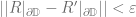
has length ![\ell(R'(s_1)) \leq 2 \sigma (d/10) m_2(R'([f_1, f_1+d/10] \times [0,\sigma]))](https://s0.wp.com/latex.php?latex=%5Cell%28R%27%28s_1%29%29+%5Cleq+2+%5Csigma+%28d%2F10%29+m_2%28R%27%28%5Bf_1%2C+f_1%2Bd%2F10%5D+%5Ctimes+%5B0%2C%5Csigma%5D%29%29&bg=ffffff&fg=5e5e5e&s=0&c=20201002) .
.![m_2(R'([f_1, f_1+d/10] \times [0,\sigma])) \leq 1](https://s0.wp.com/latex.php?latex=m_2%28R%27%28%5Bf_1%2C+f_1%2Bd%2F10%5D+%5Ctimes+%5B0%2C%5Csigma%5D%29%29+%5Cleq+1&bg=ffffff&fg=5e5e5e&s=0&c=20201002) , we have
, we have 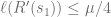 .
.
![e_2 \in [f_2 - d/10, f_2]](https://s0.wp.com/latex.php?latex=e_2+%5Cin+%5Bf_2+-+d%2F10%2C+f_2%5D&bg=ffffff&fg=5e5e5e&s=0&c=20201002) where
where 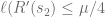 .
. by a semicircle contained in
  .
.
 still covers
  , there exists
  where
where  latex V_i$.
 the two maps
  apart, we have
  .
. .
. .
. , we will break
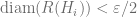
  into three parts and estimate diameter of each part separately.
 ,
,  is another parametrization of
  .
. to
to  is contained in
  , the arc in
  is
is  hence the union of the two has diameter at most
 are less than
  .
.  . By lemma, this implies the arc in
  has length at most
  .
. .
. .
.