Last Wednesday Terry Tao briefly dropped by our little town and gave a colloquium. Surprisingly this is only the second time I hear him talking (the first one goes back to undergrad years in Toronto, he talked about arithmetic progressions of primes, unfortunately it came before I learned anything [such as those posts] about Szemeredi’s theorem). Thanks to the existence of blogs, feels like I knew him much better than that!
This time he talked about Hilbert’s 5th problem, Gromov’s polynomial growth theorem for discrete groups and their (Breuillard-Green-Tao) recently proved more general analogy of Gromov’s theorem for approximate groups. Since there’s no point for me to write 2nd-handed blog post while people can just read his own posts on this, I’ll just record a few points I personally found interesting (as a complete outsider) and moving on to state the more general Hilbert-Smith conjecture, very recently solved for 3-manifolds by John Pardon (who now graduated from Princeton and became a 1-st year grad student at Stanford, also appeared in this earlier post when he gave solution to Gromov’s knot distortion problem).
Warning: As many of you know I never take notes during talks, hence this is almost purely based on my vague recollection of a talk half a week ago, inaccuracy and mistakes are more than possible.
All topological groups in this post are locally compact.
Let’s get to math~ As we all know, a Lie group is a smooth manifold with a group structure where the multiplication and inversion are smooth self-diffeomorphisms. i.e. the object has:
1. a topological structure
2. a smooth structure
3. a group structure
It’s not too hard to observe that given a Lie group, if we ‘forget’ the smooth structure and just see it as a topological group which is a (topological) manifold, then we can uniquely re-construct the smooth structure from the group structure. From my understanding, this is mainly because given any element in the topological group we can find a unique homomorphism of the group 


The way to do that is to ‘zig-zag’:
Pick a small 

The above shows that given a Lie group to start with, the smooth structure is uniquely determined by the topological group structure. Knowing this leads to the natural question:
Hilbert’s fifth problem: Is it true that any topological group which are (topological) manifolds admits a smooth structure compatible with group operations?
Side note: I had a little post-colloquium discussion with our fellow grad student Sam Lewallen, he asked:
Question: Is it possible for the same topological manifold to have two different Lie group structures where the induced smooth structures are different?
Note that neither the above nor Hilbert’s fifth problem shows such thing is impossible, since they both start with the phase ‘given a topological group’. My *guess* is this should be possible (so please let me know if you know the answer!) The first attempt might be trying to generate an exotic 

Anyways, so the Hilbert 5th problem was famously solved in the 50s by Montgomery-Zippin and Gleason, using set-theoretical methods (i.e. ultrafilters).
Gromov comes in later on and made the brilliant connection between (infinite) discrete groups and Lie groups. i.e. one see a discrete group as a metric space with word metric, ‘zoom out’ the space and produce a sequence of metric spaces, take the limit (Gromov-Hausdorff limit) and obtain a ‘continuous’ space. (which is ‘almost’ a Lie group in the sense that it’s an inverse limit of Lie groups.)
Hence he was able to adapt the machinery of Montgomery-Zippin to prove things about discrete groups:
Theorem: (Gromov) Any group with polynomial growth is virtually nilpotent.
Side note: I learned about this through the very detailed and well-presented course by Dave Gabai. (I thought I must have blogged about this, turns out I haven’t…)
The beauty of the theorem is (in my opinion) that we are given any discrete group, and all that’s known is how large the balls are (in fact, not even that, we know how large the large balls grow), yet the conclusion is all about the algebraic structure of the group. To learn more about Gromov’s work, see his paper. Although unrelated to the rest of this post, I shall also mention Bruce Kleiner’s paper where he proved Gromov’s theorem without using Hilbert’s 5th problem, instead he used space of harmonic maps on graphs.
Now we finally comes to a point of briefly mentioning the work of Tao et.al.! So they adopted Gromov’s methods of limiting and ‘ultra-filtering’ to apply to stuff that’s not even a whole discrete group: Since Gromov’s technique was to take the limit of a sequence of metric spaces which are zoomed out versions of balls in a group, but the Gromov-Hausdorff limit actually doesn’t care about the fact that those spaces are zoomed out from the same group, they may as well be just a family of subsets of groups with ‘bounded geometry’ of a certain kind.
Definition: An K-approximate group 


We shall be particularly interested in sequence of larger and larger sets (in cardinality) that are K-approximate groups with fixed
Examples:
Intervals ![[-N, N] \subseteq \mathbb{Z}](https://s0.wp.com/latex.php?latex=%5B-N%2C+N%5D+%5Csubseteq+%5Cmathbb%7BZ%7D&bg=ffffff&fg=5e5e5e&s=0&c=20201002)
Balls of arbitrarily large radius in 

Balls of arbitrarily large radius in the 3-dimensional Heisenberg group are 
Just as in Gromov’s theorem, they started with any approximate group (a special case being sequence of balls in a group of polynomial growth), and concluded that they are in fact always essentially balls in Nilpotent groups. More precisely:
Theorem: (Breuillard-Green-Tao) Any K-approximate group 


With this theorem they were able to re-prove (see p71 of their paper) Cheeger-Colding’s result that
Theorem: Any closed 
Where Gromov’s theorem yields the same conclusion only for non-negative Ricci curvature.
Random thoughts:
1. Can Kleiner’s property T and harmonic maps machinery also be used to prove things about approximate groups?
2. The covering definition as we gave above in fact does not require approximate group
As promised, I shall say a few words about the Hilbert-Smith conjecture and drop a note on the recent proof of it’s 3-dimensional case by Pardon.
From the solution of Hilbert’s fifth problem we know that any topological group that is a n-manifold is automatically equipped with a smooth structure compatible with group operations. What if we don’t know it’s a manifold? Well, of course then they don’t have to be a Lie group, for example the p-adic integer group 
Hilbert-Smith conjecture: Any topological group acting faithfully on a connected n-manifold is a Lie group.
Recall an action is faithful if the homomorphism 
As mentioned in Tao’s post, in fact
Conjecture:
The exciting new result of Pardon is that by adapting 3-manifold techniques (finding incompressible surfaces and induce homomorphism to mapping class groups) he was able to show:
Theorem: (Pardon ’12) There is no faithful action of
And hence induce the Hilbert-Smith conjecture for dimension 3.
Discovering this result a few days ago has been quite exciting, I would hope to find time reading and blogging about that in more detail soon.
 with boundary, if the inclusion map
  is not injective, then there exists a simple non-trivial loop in
  bounding an embedded disc in
  , edge set
  , to each vertex
  we associate a group
  and to each edge
  (say connecting
  ) we also associate a group
  , together with a pair of injective homomorphisms
  ,
,  .
. homeomorphic to
  , the Sierpinski carpet or the Menger curve.
 , my wonderful advisor Dave Gabai
  by isometries. (i.e. it’s almost the fundamental group of some hyperbolic surface except for possible finite order elements which make the action not properly discontinuous.)
 , we have:
 , then
  each
each  .
. with two vertices both labeled
  edges, all going from one vertex to the other. Let the edge groups be
  be a 2-complex associated to a set of generators and relations for
  be 2-complexes associated to
  . The inclusion map induces cellular maps
  . Hence we have
 be the mapping cylinder of
  . i.e.
  and
and  be the complex obtained by gluing together two copies of
  . Now the fundemental group
  of
of  is a n-dimensional Poincare duality group iff it’s torsion free and
  has integral Cech cohomology of
 IS the sphere! So it’s a 3-dimensional Poincare duality group~ Now we have a splitting of
  is a Poincare duality pair.
 is defined as
 connecting the two points.
 of the tangent bundle (depending continuously on the base point). We may attempt to define the metric
 is the collection of curves connecting
  for all
  . (i.e. we are only allowed to go along directions in the sub-bundle.
 -plane at all points. It’s easy to realize that now we are ‘stuck’ in the same height: any two points with different
  coordinate will have no curve connecting them (hence the distance is infinite). The resulting metric space is real number many discrete copies of
  . Of course that’s no longer homeomorphic to
  away from the original point
  can be connected to
  going along
  real entry Heisenberg group
  (all
(all 
 be a left-invariant metric on
  .
. (tangent space of the identity element), the elements
  and
and  form a basis.
 of the tangent bundle generated by infinitesimal left translations by
  . Since the metric
 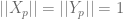 for each
  .
. .
.
 ,
, -direction stay the same, i.e. a bunch of horizontal lines connecting the original
  planes orthogonally.
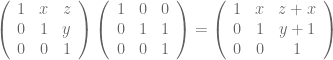
 -direction but also adds a height
 to
to  . –since going along the
 in fact up to a constant going along such loop gives the actual distance.
 ?
? in
in  . This gives
  .
. :
:
 . (A lot shorter compare to length
  for going
  , it’s much more efficient to travel in the C-C metric.
 (meaning bounded from both inside and outside with a constant factor). Hence the volume of balls grow like
  .
.
 on the plane, one needs a rope of length at least
  .” or equivalently, given
  bounded open, we always have
 :
: , we have
 is the volume of the unit n-ball. Note that the inequality is sharp for balls in
  be its Cayley graph, equipped with the word metric
  .
. be the cardinality of the ball of radius
  around the identity.
 , we define
  i.e. points that’s not in
  but there is an edge in the Cayley graph connecting it to some point in
  , then for any set
  ,
, .
. , so we have
  .
. , we look at how many elements of
  . (Here the idea being the size of the boundary can be lower bounded in terms of the length of the translation vector and the volume shifted outside the set. Hence we are interested in finding an element that’s not too far away from the identity but shifts a large volume of
  as
as  is:
is: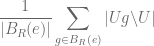
 , count how many
  outside
  .
. .
. , hence
  .
. 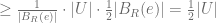
 (at least as large as average).
 .
. , since
  , there must be some
  s.t.
s.t.  and
and  .
.  ,
,  .
. i.e. a union of
  .
.

 , we have
  .
.  , hence we have
 , then trancing through the argument we get bound
 . But to get that one needs to use more information of the expander than merely the volume of balls.
 then for any open set
 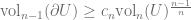 .
. is above average.
 ![\gamma: [0, ||g||]](https://s0.wp.com/latex.php?latex=%5Cgamma%3A+%5B0%2C+%7C%7Cg%7C%7C%5D&bg=ffffff&fg=5e5e5e&s=0&c=20201002) be a unit speed geodesic connecting
be a unit speed geodesic connecting ![\gamma([0, ||g||])](https://s0.wp.com/latex.php?latex=%5Cgamma%28%5B0%2C+%7C%7Cg%7C%7C%5D%29&bg=ffffff&fg=5e5e5e&s=0&c=20201002) , this must contain all of
, this must contain all of  since for any
  the segment
 ![\gamma([0,||g||]) \cdot u](https://s0.wp.com/latex.php?latex=%5Cgamma%28%5B0%2C%7C%7Cg%7C%7C%5D%29+%5Ccdot+u&bg=ffffff&fg=5e5e5e&s=0&c=20201002) must cross the boundary of
must cross the boundary of ![c \in [0,||g||]](https://s0.wp.com/latex.php?latex=c+%5Cin+%5B0%2C%7C%7Cg%7C%7C%5D&bg=ffffff&fg=5e5e5e&s=0&c=20201002) where
where  , hence
 .
.

 .
.  of
of  where there exists a k-dimensional affine subspace
  s.t. all points of
  .
.
 is the length of the orthogonal segment from
  .
. . However it is not the case since for example the equilateral triangle of side length
  . In fact, by a theorem of
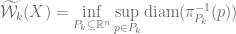
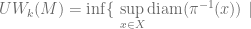
 where there is an orthogonal projection of
  has pre-image with diameter
  .
.
 .
. , unlike
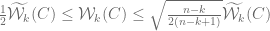
 iff
iff  where any point
  has pre-image with diameter
  .
.

 sets in the cover and
 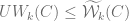 since the pair
  is clearly among the pairs we are minimizing over.
![M=[0,1]^n](https://s0.wp.com/latex.php?latex=M%3D%5B0%2C1%5D%5En&bg=ffffff&fg=5e5e5e&s=0&c=20201002) be the solid n-dimensional cube, then for any topological space
be the solid n-dimensional cube, then for any topological space  and any continuous map
  , we have image of at least one pair of opposite
  -faces intersect.
![M = [0, L_1] \times [0, L_2] \times \cdots \times [0, L_n]](https://s0.wp.com/latex.php?latex=M+%3D+%5B0%2C+L_1%5D+%5Ctimes+%5B0%2C+L_2%5D+%5Ctimes+%5Ccdots+%5Ctimes+%5B0%2C+L_n%5D&bg=ffffff&fg=5e5e5e&s=0&c=20201002) ,
,  , we have
  ; furthermore,
  for all
  ,
,  being the product of the first
  coordinates. Now
  ).
). then the notion is the same as the minimax length of fibres. In particular as proved in the post the minimax length of the unit disc to
  -disk,
 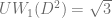 , i.e. the optimum is obtained by contracting the disc onto a triod.
 about
about  .
.