A train track on twice punctured torus

April 22, 2012April 23, 2012 Conan4 Comments

This is a non-technical post about how I started off trying to prove a lemma and ended up painting this:

One of my favorite books of all time is Thurston‘s ‘Geometry and Topology of 3-manifolds‘ (and I just can’t resist to add here, Thurston, who happen to be my academic grandfather, is in my taste simply the coolest mathematician on earth!) Anyways, for those of you who aren’t topologists, the book is online and I have also blogged about bits and parts of it in some old posts such as this one.

I still vividly remember the time I got my hands on that book for the first time (in fact I had the rare privilege of reading it from an original physical copy of this never-actually-published book, it was a copy on Amie‘s bookshelf, which she ‘robbed’ from Benson Farb, who got it from being a student of Thurston’s here at Princeton years ago). Anyways, the book was darn exciting and inspiring; not only in its wonderful rich mathematical content but also in its humorous, unserious attitude — the book is, in my opinion, not an general-audience expository book, but yet it reads as if one is playing around just to find out how things work, much like what kids do.

To give a taste of what I’m talking about, one of the tiny details which totally caught my heart is this page (I can’t help smiling each time when flipping through the book and seeing the page, and oh it still haunts me >.<):

This was from the chapter about Kleinian groups, when the term ‘train-track’ was first defined, he drew this image of a train(!) on moving on the train tracks, even have smoke steaming out of the engine:

To me such things are simply hilarious (in the most delightful way).

Many years passed and I actually got a bit more into this lamination and train track business. When Dave asked me to ‘draw your favorite maximal train track and test your tube lemma for non-uniquely ergodic laminations’ last week, I ended up drawing:

Here it is, a picture of my favorite maximal train track, on the twice punctured torus~! (Click for larger image)

Indeed, the train is coming with steam~

Since we are at it, let me say a few words about what train tracks are and what they are good for:

A train track (on a surface) is, just as one might expect, a bunch of branches (line segments) with ‘switches’, i.e. whenever multiple branches meet, they must all be tangent at the intersecting point, with at least one branch in each of the two directions. By slightly moving the switches along the track it’s easy to see that generic train track has only switches with one branch on one side and two branches on the other.

On a hyperbolic surface $S_{g,p}$ , a train track is maximal if its completementry region is a disjoint union of triangles and once punctured monogons. i.e. if we try to add more branches to a maximal track, the new branch will be redundant in the sense that it’s merely a translate of some existing branch.

As briefly mentioned in this post, train tracks give natural coordinate system for laminations just like counting how many times a closed geodesic intersect a pair of pants decomposition. To be slightly more precise, any lamination can be pushed into some maximal train track (although not unique), once it’s in the track, any laminations that’s Hausdorff close to it can be pushed into the same track. Hence given a maximal train track, the set of all measured laminations carried by the train track form an open set in the lamination space, (with some work) we can see that as measured lamination they are uniquely determined by the transversal measure at each branch of the track. Hence giving a coordinate system on $\mathcal{ML})(S)$ .

Different maximal tracks are of course them pasted together along non-maximal tracks which parametrize a subspace of $\mathcal{ML}(S)$ of lower dimension.

To know more about train tracks and laminations, I highly recommend going through the second part of Chapter 8 of Thurston’s book. I also mentioned them for giving coordinate system on the measured lamination space in the last post.

In any case I shall stop getting into the topology now, otherwise it may seem like the post is here to give exposition to the subject while it’s actually here to remind myself of never losing the Thurston type childlike wonder and imagination (which I found strikingly larking in contemporary practice of mathematics).

Haken manifolds and virtual Haken conjecture

November 21, 2011November 22, 2011 Conan1 Comment

Hi people~ My weekends have been unfortunately filled up with grading undergrad assignments for the last couple of weeks >.< I'll try to catch up on blogging by finding some other time slot during the week.

As a grand-student of Thurston's I feel obligated to end my ignorance regarding Haken manifolds. I guess it's a good idea to start by writing my usual kids-friendly exposition here.

In the rest of the post, $M$ is a compact (so perhaps with boundary), orientable, irreducible (meaning each embedded 2-sphere bounds a ball) 3-manifold.

Definition: A properly embedded oriented surface $S \subseteq M$ is incompressible if $S$ is not the 2-sphere and any simple closed curve on $S$ which bounds an embedded disc in $M \backslash S$ also bounds one in $S$ .

Figure 1

In other words, together with Dehn’s lemma this says the map $\varphi: \pi_1(S) \rightarrow \pi_1 (M)$ induced by the inclusion map is injective.

Note that the surface $S$ could have boundary, for example:

Figure 2

Definition: $M$ is Haken if it contains an incompressible surface.

Okay, at this point you should be asking, what’s good about Haken manifolds? The beauty about it is that, roughly speaking, once you find one incompressible surface in the manifold, you can just keep finding them until the manifold is completely chopped up into balls by incompressible surfaces.

Theorem: (Haken) Any Haken 3-manifold $M$ contains a hierarchy $S_0 \subseteq S_1 \subseteq \cdots \subseteq S_n$ where

1. $S_0$ is an incompressible surface in $M$
2. $S_i = S_{i-1} \cup S$ where $S$ is an incompressible surface for the closure of some connected component $K$ of $latex $M \backslash S_{i-1}$
3. $M \backslash S_n$ is a union of 3-balls

Sketch of proof: This is much simpler than it might appear to be. The point is (at least in my opinion), except for trivial cases as long as a manifold has boundary it must be Haken.

Lemma: If $\partial M$ has a component that’s not $\mathbb{S}^2$ then $M$ is Haken.

The proof of the lemma is merely that any such $M$ will have infinite $H_2$ hence by the sphere theorem it will contain an embedded surface with non-trivial homology, if such surface is compressible then we just cut along the boundary of the compressing disc and glue two copies of it. This does not change the homology. Hence at the end we will arrive at a non-trivial incompressible surface.

Figure 3

Now back to proving of the theorem, so we start by setting $S_0$ to be an incompressible surface given by $M$ being Haken.

Now since $M$ is irreducible, we cut along $S_0$ , i.e. take the closure of each component (may have either one or two components) of $M\backslash S_0$ . Those will have a non-spherical boundary component, hence by lemma containing homologically non-trivial incompressible surface.

This process continuous as long as some pieces has non-spherical boundary components. But since $M$ is irreducible, any sphere bounds a 3-ball in $M$ , hence all components with sphere boundary are 3-balls. (In particular, the case where a component have multiple sphere boundary components cannot occur since the first boundary component bounds a 3-ball hence it can’t have any non-trivial incompressible surfaces on both sides.)

Now the only remaining piece is to show that this process terminates. We apply a standard ‘normal surface argument’ for this. Essentially if we fix a triangulation of $M$ ,

A normal surface in $M$ is one that intersects each 3-simplex in a disjoint union of following two shapes:

Figure 4

There can’t be infinitely many non-parallel disjoint normal surfaces in $M$ (in fact there can be no more than 6 times the number of 3-simplexes since each complementry component need to contain at least one non-I-bundle part from one 3-simplex).

Figure 5

However, if the above process do not terminate, we would obtain a sequence of non-parallel non-spherical boundary components:

Figure 6

They represent different homology classes hence can be represented by disjoint normal which results in a contradiction.

In general, this gives a way to prove theorems about Haken manifolds by using inductionL i.e. one may hope to just show the property trivially holds for 3-balls and is invariant under gluing two pieced along an incompressible surface. Note that the gluing surface being incompressible is in fact quite strong hence making the induction step possible in many cases.

For example, by applying an incredible amount of brilliant techniques, Thurston was able to prove his revolutionary result:

Hyperbolization theorem for Haken manifolds: Any Haken manifold $M$ with tori boundary components that does not contain incompressible tori admits a complete hyperbolic structure of finite volume in its interior.

In other words, this is saying that given a Haken manifold, we cut along any incompressible tori, the resulting manifold with tori boundary must have a complete hyperbolic structure with cusps near each boundary component,

This is the best we could hope for since manifolds with incompressible tori would have their fundamental group split over $Z^2$ which of course imply they can’t be hyperbolic.

Now the more manifolds being Haken means the better this theorem is. Many evidences show that in fact a lot of manifolds are indeed Haken, in perticular we have:

Virtual Haken Conjecture: $M$ is finitely covered by a Haken manifold as long as $\pi_1(M)$ is infinite.

We can see that together with Thurston’s hyperbolization theorem, this would give full solution to the geometrization conjecture for general 3-manifolds.

However, although now Perelman has proved the geometrization conjecture, the virtual Haken conjecture remains open. But in light of Perelman’s result now we are able to try to ‘back-solve’ the puzzle and only prove the virtual Haken conjecture for hyperbolic manifolds.

(to be continued)

A report from the Workshop in Geometric Topology @ Utah (part 1)

May 29, 2011June 13, 2011 Conan9 Comments

I went to Park City this passed week for the Workshop in Geometric Topology. It was a quite cool place filled with ski-equipment stores, Christmas souvenir shops, galleries and little wooden houses for family winter vacations. Well, as you may have guessed, the place would look very interesting in summer. :-P

As the ‘principal speaker’, Professor Gabai gave three consecutive lectures on his ending lamination space paper (this paper was also mentioned in my last post). I would like to sketch some little pieces of ideas presented in perhaps couple of posts.

Classification of simple closed curves on surfaces

Let $S_{g,p}$ denote the (hyperbolic) surface of genus $g$ and $p$ punchers. There is a unique geodesic loop in each homotopy class. However, given a geodesic loop drew on the surface, how would you describe it to a friend over telephone?

Here we wish to find a canonical way to describe homotopy classes of curves on surfaces. This classical result was originally due to Dehn (unpublished), but discovered independently by Thurston in 1976. For simplicity let’s assume for now that $S$ is a closed surface of genus $g$ .

Fix pants decomposition $\mathcal{T}$ of $S$ , $\mathcal{T} = \{ \tau_1, \tau_2, \cdots, \tau_{3g-3} \}$ is a disjoint union of $3g-3$ ‘cuffs’.

As we can see, any simple closed curve will have an (homology) intersection number with each of the cuffs. Those numbers are non-negative integers:

Around each cuff we may assign an integer twist number, for a cuff with intersection number $n$ and twist number $z$ , we ‘twist’ the curve inside a little neighborhood of the cuff so that all transversal segments to the cuff will have $z$ intersections with the curve.

Negative twists merely corresponds to twisting in the other direction:

Theorem: Every simple closed curve is uniquely defined by its intersection number and twisting number w.r.t each of the cuffs.

Conversely, if we consider multi-curves (disjoint union of finitely many simple closed curves) then any element in $\mathbb{Z}^{3g-3} \times \mathbb{Z}_{\geq 0}^{3g-3}$ describes a unique multi-curve.

To see this we first assume that the pants decomposition comes with a canonical ‘untwisted’ curve connecting each pairs of cuffs in each pants. (i.e. there is no god given ‘0’ twist curves, hence we have to fix which ones to start with.)

In the example above our curve was homotopic to the curve $((1,2), (2,1), (1,-4))$ .

In other words, pants decompositions (together with the associated 0-twist arcs) give a natural coordinate chart to the set of homotopy class of (multi) curves on a surface. i.e. they are perimetrized by $\mathbb{Z}^{3g-3} \times \mathbb{Z}_{\geq 0}^{3g-3}$ .

For the converse, we see that any triple of integers can be realized by filling the pants with a unique set of untwisted arcs:

In fact, this kind of parametrization can be generalized from integers to real numbers, in which case we have measured laminations instead of multi-curves and maximal train trucks on each pants instead of canonical untwisted arcs. i.e.

Theorem: (Thurston) The space of measured laminations $\mathcal{ML}(S)$ on a surface $S$ of genus $g$ is parametrized by $\mathbb{R}^{3g-3} \times \mathbb{R}_{\geq 0}^{3g-3}$ . Furthermore, the correspondence is a homeomorphism.

Here the intersection numbers with the cuffs are wrights of the branches of the train track, hence it can be any non-negative real number. The twisting number is now defined on a continuous family of arcs, hence can be any real number, as shown below:

As we can see, just as in the case of multi-curves, any triple of real numbers assigned to the cuffs can be realized as the weights of branches of a train track on the pants.

Stabilization of Heegaard splittings

May 9, 2011May 14, 2011 ConanLeave a comment

In the last lecture of a course on Heegaard splittings, professor Gabai sketched an example due to Hass-Thompson-Thurston of two genus $g$ Heegaard splittings of a $3$ -manifold that requires at least $g$ stabilization to make them equivalent. The argument is, in my opinion, very metric-geometric. The connection is so striking (to me) so that I feel necessary to give a brief sketch of it here.

(Side note: This has been a wonderful class! Although I constantly ask stupid questions and appear to be confused from time to time. But in fact it has been very interesting! I should have talked more about it on this blog…Oh well~)

The following note is mostly based on professor Gabai’s lecture, I looked up some details in the original paper ( Hass-Thompson-Thurston ’09 ).

Recall: (well, I understand that I have not talked about Heegaard splittings and stabilizations here before, hence I’ll *try to* give a one minute definition)

A Heegaard splitting of a 3-manifold $M$ is a decomposition of the manifold as a union of two handlebodies intersecting at the boundary surface. The genus of the Heegaard splitting is the genus of the boundary surface.

All smooth closed 3-manifolds has Heegaard splitting due the mere existence of a triangulation ( by thicken the 1-skeleton of the triangulation one gets a handlebody perhaps of huge genus, it’s easy exercise to see its complement is also a handlebody). However it is of interest to find what’s the minimal genus of a Heegaard splitting of a given manifold.

Two Heegaard splittings are said to be equivlent if there is an isotopy of the manifold sending one splitting to the other (with boundary gluing map commuting, of course).

A stabilization of a Heegaard splitting $(H_1, H_2, S)$ is a surgery on $S$ that adds genus (i.e. cut out two discs in $S$ and glue in a handle). Stabilization will increase the genus of the splitting by $1$ )

Let $M$ be any closed hyperbolic $3$ -manifold that fibres over the circle. (i.e. $M$ is $F_g \times [0,1]$ with the two ends identified by some diffeomorphism $f: F_g \rightarrow F_g$ , $g\geq 2$ ):

Let $M'_k$ be the $k$ fold cover of $M$ along $S^1$ (i.e. glue together $k$ copies of $F_g \times I$ all via the map $f$ :

Let $M_k$ be the manifold obtained by cut open $M'_k$ along $F_g$ and glue in two handlebodies $H_1, H_2$ at the ends:

Since $M$ is hyperbolic, $M'_k$ is hyperbolic. In fact, for any $\varepsilon > 0$ we can choose a large enough $k$ so that $M_k$ can be equipped with a metric having curvature bounded between $1-\varepsilon$ and $1+\varepsilon$ everywhere.

( I’m obviously no in this, however, intuitively it’s believable because once the hyperbolic part $M'_k$ is super large, one should be able to make the metric in $M'_k$ slightly less hyperbolic to make room for fitting in an almost hyperbolic metric at the ends $H_1, H_2$ ). For details on this please refer to the original paper. :-P

Now there comes our Heegaard splittings of $M_k$ !

Let $k = 2n$ , let $H_L$ be the union of handlebody $H_1$ together with the first $n$ copies of $M$ , $H_R$ be $H_2$ with the last $n$ copies of $M$ . $H_L, H_R$ are genus $g$ handlebodies shearing a common surface $S$ in the ‘middle’ of $M_k$ :

Claim: The Heegaard splitting $\mathcal{H}_1 = H_L \cup H_R$ and $\mathcal{H}_2 = H_L \cup H_R$ cannot be made equivalent by less than $g$ stabilizations.

In other words, first of all one can not isotope this splitting upside down. Furthermore, adding handles make it easier to turn the new higher genus splitting upside down, but in this particular case we cannot get away with adding anything less than $g$ many handles.

Okay, not comes the punchline: How would one possible prove such thing? Well, as one might have imagined, why did we want to make this manifold close to hyperbolic? Yes, minimal surfaces!

Let’s see…Suppose we have a common stabilization of genus $2g-1$ . That would mean that we can sweep through the manifold by a surface of genus (at most) $2g-1$ , with $1$ -skeletons at time $0, 1$ .

Now comes what professor Gabai calls the ‘harmonic magic’: there is a theorem similar to that of Pitts-Rubinstein

Ingredient #1: (roughly thm 6.1 from the paper) For manifolds with curvature close to $-1$ everywhere, for any given genus $g$ Heegaard splitting $\mathcal{H}$ , one can isotope the sweep-out so that each surface in the sweep-out having area $< 5 \pi (g-1)$ .

I do not know exactly how is this proved. The idea is perhaps try to shrink each surface to a ‘minimal surface’, perhaps creating some singularities harmless in the process.

The ides of the whole arguement is that if we can isotope the Heegaard splittings, we can isotope the whole sweep-out while making the time- $t$ sweep-out harmonic for each $t$ . In particular, at each time there is (at least) a surface in the sweep-out family that divides the volume of $M'_n$ in half. Furthermore, the time 1 half-volume-surface is roughly same as the time 0 surface with two sides switched.

We shall see that the surfaces does not have enough genus or volume to do that. (As we can see, there is a family of genus $2g$ surface, all having volume less than some constant independent of $n$ that does this; Also if we have ni restriction on area, then even a genus $g$ surface can be turned.)

Ingredient #2: For any constant $K$ , there is $n$ large enough so no surfaces of genus $<g$ and area $<K$ inside the middle fibred manifold with boundary $M'_n$ can divide the volume of $M'_n$ in half.

The prove of this is partially based on our all-time favorite: the isoperimetric inequality:

Each Riemannian metric $\lambda$ on a closed surface has a linear isoperimetric inequality for 1-chains bounding 2-chains, i.e. any homologically trivial 1-chain $c$ bounds a $2$ chain $z$ where

$\mbox{Vol}_2(z) \leq K_\lambda \mbox{Vol}_1(c)$ .

Fitting things together:

Suppose there is (as described above) a family of genus $2g-1$ surfaces, each dividing the volume of $M_{2n}$ in half and flips the two sides of the surface as time goes from $0$ to $1$ .

By ingredient #1, since the family is by construction surfaces from (different) sweep-outs by ‘minimal surfaces’, we have $\mbox{Vol}_2(S_t) < 5 \pi (2g-2)$ for all $t$ .

Now if we take the two component separated by $S_t$ and intersect them with the left-most $n$ copies of $M$ in $M'_{2n}$ (call it $M'_L$ ), at some $t$ , $S_t$ must also divide the volume of $M'_L$ in half.

Since $S_t$ divides both $M'_2n$ and $M'_L$ in half, it must do so also in $M'_R$ .

But $S_t$ is of genus $2g-1$ ! So one of $S_t \cap M'_L$ and $S_t \cap M'_R$ has genus $< g$ ! (say it's $M'_L$ )

Apply ingredient #2, take $K = 5 \pi (2g-2)$ , there is $n$ large enough so that $S_t \cap M'_L$ , which has area less than $K$ and genus less than $g$ , cannot possibly divide $M'_L$ in half.

Contradiction.

A convergence theorem for Riemann maps

January 17, 2011November 1, 2011 ConanLeave a comment

So~ After 2.5 weeks of wonderful math discussions with Amie and Charles, I finished my winter vacation and got back to Princeton! (and back to my normal blogging Sundays ^^)

One thing I would like to shear here is that we (me and Charles) finally got an answer to the following question that’s been haunting me for a while:

Question: Given Jordan curve $C \subseteq \mathbb{C}$ containing a neighborhood of $\bar{0}$ in its interior. Given parametrizations $\gamma_1:S^1 \rightarrow C$ .

Is it true that for all $\varepsilon >0$ , there exists $\delta >0$ s.t. any Jordan curve $C'$ with a parametrization $\gamma_2:S^1 \rightarrow C_2$ so that $||\gamma_1-\gamma_2||<\delta$ in the uniform norm implies the Riemann maps $R, R'$ from $\mathbb{D}$ to the interiors of $C, C'$ that fixes the origin and have positive real derivatives at $\bar{0}$ would be at most $\varepsilon$ apart?

i.e. Is the projection map from the space of parametrized Jordan curves (with the uniform metric) to the space of unparametrized Jordan curves (with metric given by taking uniform distance between the canonical Riemann maps) continuous?

First, I think the development and problem-solving process for this one is quite interesting and worth mentioning (skip this if you just want to see math):

—Begin story—

The problem was initially of interest because I stated a lemma on our Jordan curves paper which asserts the above projection map is continuous at smooth curves. To my surprise, I was unable to prove this seemingly-direct lemma. I turned to Charles for help, after a day or so of thinking he proved it for smooth curves (via a very clever usage of cross-cuts as in the proof of Carathedory’s theorem) and asked back whether the map is actually continuous at all points.

This seemed to be such a natural question but we couldn’t find it in the literature. For a day or so we were both feeling negative about this since the cross-cut method fails when the Jordan curve has positive measure, which “should” happen a lot. In any case, I posted a question on mathoverflow to see if there is a standard theorem out there implying this. Almost right after I posted the question, during a wonderful lunch-conversation with Charles, I got this wonderful idea of applying extremal length techniques not to the semi-circular crosscut but only to the ‘feet’ of it. Which later that day turned out to be a proof of the continuity.

The next morning, after confirming the steps of the proof and made sure it works, I was thrilled to find that Thurston responded to the post and explained his intuition that the answer is positive. Although having solved the problem already, I am still amazed by his insights ^^ (It’s the second question I asked there, he left an comment again! It just feels great to have your idol giving you ideas, isn’t it? :-P)

Later on, McMullen pointed out to us that in fact a book by Pommerenke contains the result. Nevertheless, it was great fun proving this, hence I decided to sketch the proof here ^^

—End story—

Ingredients of the proof: We quote the following well-known but weaker theorem (one can find this in, for example Goluzin’s classical book, p228)

Theorem: If the Jordan domains converge (in the sense that parametrizations of the boundaries converge uniformly) then the Riemann maps converge uniformly on compact sets.

We also use the following topological lemma:

Lemma: Given Jordan curve $C \subseteq \hat{\mathbb{C}}$ , $\gamma: S^1 \rightarrow C$ be a parametrization. For all $\varepsilon > 0$ , there exists $\mu >0$ s.t. for all $\gamma' : S^1 \rightarrow \hat{\mathbb{C}}$ with $|| \gamma - \gamma'|| < \mu$ ( denote C' = \gamma'(S^1)$) , for all $p, q \in C'$ , $d(p,q) < \mu \Rightarrow \mbox{diam}(A(p,q)) < \varepsilon$

where $A(p,q)$ is the short arc in $C'$ connecting $p, q$ .

The proof of the lemma is left as an exercise

Proof of the Theorem:

Given $C$ and $\varepsilon$ as in the theorem, apply the lemma to $(C, \varepsilon/6)$ , we obtain a $\mu < \varepsilon / 6$ so that all curves $\mu$ -close to $C$ has the property that the arc connecting any two points less than $\mu$ -apart has diameter no more than $\varepsilon/100$ .

By compactness of $\partial \mathbb{D}$ , we can choose finitely many crosscut neignbourhoods $\{ H_1, H_2, \cdots, H_N \}$ , $H_i \subseteq \bar{\mathbb{D}}$ are "semi-discs" around points in $\partial \mathbb{D}$ as shown:

By extremal length, we can choose the cross-cuts $C_i$ bounding $H_i$ with length $\ell(R(C_i)) < \mu/4$ where $R: \bar{\mathbb{D}} \rightarrow \hat{\mathbb{C}}$ is the canonical Riemann map corresponding to $C$ . Hence by lemma, we also get $\mbox{diam}(R(H_i) < \varepsilon/3$ .

Let $\{ f_1, f_2, \cdots, f_{2N} \}$ be endpoints of $\{C_1, \cdots, C_N \}$ .

Let $d = \min \{ d(f_i, f_j) \ | \ 1 \leq i < j \leq 2N \}$ .

Choose $\sigma < \mu d / 40$ and $\{ B( \bar{0}, 1-2\sigma), H_1, \cdots, H_N \}$ covers $\bar{\mathbb{D}}$ . Let $R = 1-\sigma$ :

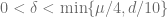
By the above theorem in Goluzin, since $B_R = \bar{B(0, R)}$ is compact, there exists a $0 < \delta < \min \{\mu/4, d/10 \}$ s.t.

$|| \gamma' - \gamma || < \delta$ $\Rightarrow ||R|_{B_R} - R'|_{B_R}|| < \mu/4$ .

Fix a $(C', \gamma')$ with $|| \gamma - \gamma'|| < \delta$ . Let $R'$ be the canonical Riemann map corresponding to $C'$ .

Claim: $||R-R'|| < \varepsilon$ .

First note that assuming the theorem in Goluzin, it suffice to show $||R|_{\partial \mathbb{D}} - R'|_{\partial \mathbb{D}}|| < \varepsilon$ .

For any $1 \leq i \leq N$ , let $f_1, f_2$ be endpoints of $C_i$ . Apply the extremal length to the set of radial segments in the almost-rectangle $[f_1, f_1+d/10] \times [0,\sigma]$ .

We conclude there exists $e_1 \in [f_1, f_1+d/10]$ s.t. the segment $s_1 = \{e_1\} \times [0, \sigma]$ has length

$\ell(R'(s_1)) \leq 2 \sigma (d/10) m_2(R'([f_1, f_1+d/10] \times [0,\sigma]))$ .

Since $\sigma < \mu d / 40$ and $m_2(R'([f_1, f_1+d/10] \times [0,\sigma])) \leq 1$ , we have

$\ell(R'(s_1)) \leq \mu/4$ .

Similarly, find $e_2 \in [f_2 - d/10, f_2]$ where $\ell(R'(s_2)\leq \mu/4$ .

Connect $e'_1, e'_2$ by a semicircle contained in $H_i$ , denote the enclosed region by $V_i \subseteq H_i$ .

By construction, $\{ B_R, V_1, \cdots, V_N \}$ still covers $\bar{\mathbb{D}}$ .

Hence for all $p \in \partial \mathbb{D}$ , there exists $i$ where $p \in$ latex V_i$.

Since inside $V_i \cap B_R$ the two maps $R, R'$ are less than $d/10$ apart, we have $R(V_i) \cap R'(V_i) \neq \phi$ .

Hence $d(R(p), R'(p)) \leq \mbox{diam}(R(H_i)) + \mbox{diam}(R'(V_i))$ .

By construction, $\mbox{diam}(R(H_i)) < \varepsilon/2$ .

$\mbox{diam}(R'(V_i)) = \mbox{diam}(\partial V_i)$ , we will break $\partial V_i$ into three parts and estimate diameter of each part separately.

Since $||\gamma-\gamma'|| < \delta$ , $\tau = \gamma' \circ \gamma^{-1} \circ R|_{\partial \mathbb{D}}$ is another parametrization of $C'$ with $|| \tau - R|_{\partial \mathbb{D}}|| < \delta$ .

The arc connecting $e'_1$ to $e'_2$ is contained in $B_R \cap V_i$ , the arc in $C'$ connecting $\tau(e_1), \tau(e_2)$ is $\delta$ away from $R(H_i)$ hence the union of the two has diameter at most $\mbox{diam}(R(V_i)) + \delta < \varepsilon/6 + \varepsilon/6 = \varepsilon/3$

Length of the arcs $R'(s_1), R'(s_2)$ are less than $\mu/4 < \varepsilon/12$ .

Hence $d(\tau(e_1), R'(e_1)) < \ell(R'(s_1)) + \delta < \mu$ . By lemma, this implies the arc in $C'$ connecting $\tau(e_1), R'(e_1)$ has length at most $\varepsilon/12$ .

Hence altogether the we have $\mbox{diam}(R'(V_i)) \leq \varepsilon/3+\varepsilon/12+\varepsilon/12 = \epsilon/2$ .

We deduce $d(R(p), R'(p)) \leq \mbox{diam}(R(H_i)) + \mbox{diam}(R'(V_i)) < \varepsilon$ .

Q.E.D.

Area777

Chasing dreams from mathematics to the real world

Tag: Thurston

A train track on twice punctured torus

Haken manifolds and virtual Haken conjecture

A report from the Workshop in Geometric Topology @ Utah (part 1)

Stabilization of Heegaard splittings

A convergence theorem for Riemann maps

Share this:

Share this:

Share this:

Share this:

Share this: