Enough of the ‘trying to understand recent big theorems’ on this blog, let’s do something light and fun this week!
As I was browsing the ArXiv one day, one thing led to anther and I eventually arrived in a very short and cute paper of Greg Kuperberg and Oded Schramm.
So, we have sphere packings, which is simply a bunch of spheres (say in 

We can associate a graph to a sphere packing with vertices representing spheres and join two vertices with an edge if two sphere kisses:

Question: What kind of graph can appear this way?
Now if we go back to two-dimensions, it’s a classical theorem that any planar graph can appear as the nerve of a circle packing. (In fact, as mentioned at the end of this earlier post, something much stronger is true. i.e. it’s a theorem of Schramm that one can ‘kiss’ pretty much any given set of planar objects with a given nerve.)
In light of this, it’s nature to wonder whether every graph can be realized as a nerve of some sphere packing (since all graph embeds in some oriented surface which then embeds in
However I would imagine it’s not easy to show things such as a given graph cannot be realized. In the paper they came up with what’s perhaps the first restriction that shows not all graphs can be realized in such packing, namely:
The average kissing number is, as one might expect, in average how many kisses does each sphere get, i.e.
2 * number of tangency points / number of balls

If one thinks about it, how might one attempt to construct a packing with super large average kissing number? Well, perhaps we start with a single sphere, put a huge amount of small spheres around it (because one cannot fit many large spheres), then this middle one does get a lot of kisses, but what about the smaller ones? If they are equal sized then all the small spheres only gets roughly 7 kisses…now we need to put even smaller spheres around each of those…If we stop at any stage, there would be more smallers spheres that’s not taken care of than the larger ones with lots of kisses, so it’s not clear at all if the average can blow up.
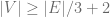
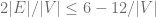
As usual, things are much simpler in two dimensions: Since the Euler characteristic of any planar graph is 2 (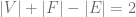


On the other hand, for our all-time favorite hexagonal packing of congruent circles, if we take more and more layers, the number of balls with six kisses grow like 


Hexagonals are the best, as expected~
Now comes what’s in the paper: they showed that for any sphere packing, the average kissing number is less than 
For simplicity I’ll only reproduce the ‘warm-up case’ in the paper which proves the kissing number is no more than 24. (well, since our goal here is only to say that not all graphs can be realized.) I find this observation (due to Schramm) is very simple, cute, and works in any dimensions.
Let’s first define some numbers:


Let 


Theorem: 
Given a sphere packing 


Define map 

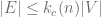
Since each sphere can only be surrounded by 


How simple!
Now going from 24 to 

Now if we look at each pair of balls, say take pair (V_1, V_2), it turns out that if they kiss, the fraction of shell around 

Hence we get a relation 

So we know 
 , for any
  , there exists
  depending only on
  such that any normed vector space of dimension
  into the Hilbert space.
 ) for any given k, *any* norm on a vector space of sufficiently high dimension will have a
  dimensional subspace that looks almost Eculidean (meaning unit ball is round up to a multiple
  ).
). , does there exist a
  so that every metric space of Hausdorff dimension
  has a subset
  of Hausdorff dimension
  that embeds into the Hilbert space with distorsion
  such that for any
  , every compact metric space with dimension
  that admits an embedding into Hilbert space with distorsion
  .
. of course blows up to infinity whenever
  or
or  . (whenever we need a huge dimensional space with fixed ‘flatness’ or a fixed dimension but ‘super-flat’ subspace). That is, when we are looking for subspaces inside a random space with fixed (large) dimension
  necessarily forces
  and
and .
. ), but not so great when we want small distorsion (it does not apply when distorsion is smaller than
  ! In fact, when we are allowing relatively large distorsion (compare to constant
  and a family of metric spaces
  such that for any small
  , no subset of
  with dimension
  embeds into Hilbert space with distorsion
  .
. , there is no
  , in the paper they also produced spaces
  are of Hausdorff dimension 0!
 is a metric with the additional property that for any three points
  , we have the so-called strong triangle inequality, i.e.
 , with the dictionary metric (two points are distance
  apart where
  . It’s not hard to see in fact all such space embeds isometrically in
  by a Lipschitz map.