A few weeks ago, I received this mysterious e-mail invitation to the ‘Oxtoby Centennial Conference’ in Philadelphia. I had no idea about how did they find me since I don’t seem to know any of the organizers, as someone who loves conference-going, of course I went. (Later I figured out it was due to Mike Hockman, thanks Mike~ ^^ ) The conference was fun! Here I want to sketch a few cool items I picked up in the past two days:
Definition:A Borel measure 
![[0,1]^n](https://s0.wp.com/latex.php?latex=%5B0%2C1%5D%5En&bg=ffffff&fg=5e5e5e&s=0&c=20201002)
i)
ii)
iii)
iv)
![\mu([0,1]^n) = 1](https://s0.wp.com/latex.php?latex=%5Cmu%28%5B0%2C1%5D%5En%29+%3D+1&bg=ffffff&fg=5e5e5e&s=0&c=20201002)
![\mu(\partial [0,1]^n) = 0](https://s0.wp.com/latex.php?latex=%5Cmu%28%5Cpartial+%5B0%2C1%5D%5En%29+%3D+0&bg=ffffff&fg=5e5e5e&s=0&c=20201002)
Oxtoby-Ulam theorem:
Any Oxtoby-Ulam measure is the pull-back of the Lebesgue measure by some homeomorphism ![\phi: [0,1]^n \rightarrow [0,1]^n](https://s0.wp.com/latex.php?latex=%5Cphi%3A+%5B0%2C1%5D%5En+%5Crightarrow+%5B0%2C1%5D%5En&bg=ffffff&fg=5e5e5e&s=0&c=20201002)
i.e. For any Borel set ![A \subseteq [0,1]^n](https://s0.wp.com/latex.php?latex=A+%5Csubseteq+%5B0%2C1%5D%5En&bg=ffffff&fg=5e5e5e&s=0&c=20201002)

It’s surprising that I didn’t know this theorem before, one should note that the three conditions are clearly necessary: A homeo has to send open sets to open sets, points to points and boundary to boundary; we know that Lebesgue measure is positive on open sets, 
Since I came across this at such a late time, my first reaction was: this is like Moser’s theorem in the continuous case! But much cooler! Because measures are a lot worse than differential forms: many weird stuff could happen in the continuous setting but not in the smooth setting.
For example, we can choose a countable dense set of smooth Jordan curves in the cube and assign each curve a positive measure (we are free to choose those values as long as they sum to 

Question: (posed by Albert Fathi, 1970)
Does the homeomorphism 
My first thought was to use smooth volume forms to approximate the measure, for smooth volume forms, Moser’s theorem gives diffeomosphisms depending continuously w.r.t. the form (I think this is true just due to the nature of the construction of the Moser diffeos) the question is how large is the closure of smooth forms in the space of OU-measures. So I raised a little discussion immediately after the talk, as pointed out by Tim Austin, under the weak topology on measures, this should be the whole space, with some extra points where the diffeos converge to something that’s not a homeo. Hence perhaps one can get the homeo depending weakly continuously on
Lifted surface flows:
Nelson Markley gave a talk about studying flows on surfaces by lifting them to the universal cover. i.e. Let 


There is an early result:
Theorem: (Weil) Let 


i.e. for lifted flows, if an orbit escapes to infinity, then it must escape along some direction. (No sprial-ish or wild oscillating behavior) This is due to the nature that the flow is the same on each unit square.
We can find its analogue for surfaces with genus larger than one:
Theorem: Let 


Using those facts, they were able to prove results about the structure of 
I was curious about what kind of orbits (or just non-self intersecting curves) would ‘escape’, so here’s some very simple observations: On the torus, this essentially means that the curve does not wind around back and forth infinitely often with compatible magnitudes, along both generators. i.e. the curve ‘eventually’ winds mainly in one direction along each generating circle. Very loosely speaking, if a somewhat similar thing is true for higher genus surfaces, i.e. the curve eventually winds around generators in one direction (and non-self intersecting), then it would not be able to have very complicated
Measures on Cantor sets
In contrast to the Oxtoby-Ulam theorem, one could ask: Given two measures on the standard middle-third Cantor set, can we always find a self homeomorphism of the Cantor set, pushing one measure to the other?
Given there are so many homeomorphisms on the Cantor set, this sounds easy. But in fact it’s false! –There are countably many clopen subsets of the Cantor set (Note that all clopen subsets are FINITE union of triadic copies of Cantor sets, a countable union would necessarily have a limit point that’s not in the union), a homeo needs to send clopen sets to clopen sets, hence for there to exist a homeo the countably many values the measures take on clopen sets must agree.
So a class of ‘good measures’ on Cantor sets was defined in the talk and proved to be realizable by a pull back the standard Hausdorff measure via a homeo.
I was randomly thinking about this: Given a non-atomic measure
In any case, it’s been a fun weekend! ^^
 be a diffeomorphism. A point
  is non-wandering if for all neighborhood
  of
of  where
where  . We write
  .
. there exists diffeomorphism
  s.t.
s.t.  and
and  for some
  .
. is compact, then for any
  ,
,  s.t.
s.t.  .
. .
. where
where
 or
or  . Iterate the above process. since the sequence is at least one term shorter after each shortening, the process stops in finite time. We obtain final sequence
  s.t. for all
  ,
, .
. times,
  , after the first shortening,
 .
. . Along the same line, we have, at the
  -th shortening, the distance between the initial and final sequence and
  . Hence for the final sequence
  .
. where
where 
 by a factor of
  w.r.t. the center) and for all
  .
. in
in  with
with  and
and  id. Hence
 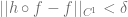 .
. are the lengths of
  ,
,  .
. .
. , it's at least
  away from the boundary of
  satisfying the above condition and
  .
. , we need about
  such bump functions, to move a distance
  , we need about
  bumps.
 is a surface. By starting with an
  (and hence
  is contained in a small neighbourhood of
  . Hence on
  is
is  close to the linear map
  . Hence mod some details we may reduce to the case where
  .
. ,
,  has height greater than width. (note that
  bumps will be able to move the point by a distance equal to the width of the original rectangle
  s.t. for all
  ,
,  , the boxes
  . Construct
 has the property that
  lies on the same vertical fiber as
  .
. , we let
 ,
,  .
. 
 .
. of
of  , we may further perturb
  be its time-1 map. Consider a
  perturbation of
  . We are interested in when is the perturbed map still a time-1 map of a flow.