This is one of those items I should have written about long ago: I first heard about it over a lunch chat with professor Guth; then I was in not one, but two different talks on it, both by Peter Jones; and now, finally, after it appeared in this algorithms lecture by Sanjeev Arora I happen to be in, I decided to actually write the post. Anyways, it seem to live everywhere around my world, hence it’s probably a good idea for me to look more into it.
Has everyone experienced those annoy salesman who keeps knocking on you and your neighbors’ doors? One of their wonderful properties is that they won’t stop before they have reached every single household in the area. When you think about it, in fact this is not so straight foreword to do; i.e. one might need to travel a long way to make sure each house is reached.
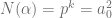
Problem: Given 


Since this started as an computational complexity problem (although in fact I learned the analysts’s version first), I will mainly focus on the CS version.
Trivial observations:
In total there are about 

This can be easily improved by a standard divide and concur:
Let 


Now the value of this 


Otherwise

What we need is minimum of 


Can we make it polynomial time? No. It’s well known that this problem is NP-hard, this is explained well in the wikipedia page for the problem.
Well, what can we do now? Thanks to Arora (2003), we can do an approximate version in polynomial time. I will try to point out a few interesting ideas from that paper. The process involved in this reminded me of the earlier post on nonlinear Dvoretzky problem (it’s a little embracing that I didn’t realize Sanjeev Arora was one of the co-authors of the Dvoretzky paper until I checked back on that post today! >.< ) it turns out they have this whole program about ‘softening’ classic problems and produce approximate versions.
Approximate version: Given 


Of course we shall expect the running time 


The above is what I would hope is proved to be polynomial. In reality, what Arora did was one step more relaxed, namely a polynomial time randomized approximate algorithm. i.e. Given 

Theorem (Arora ’03): 
Later in that paper he improved the bound to 
Selected highlights of proof:
One of the great features in the approximating world is that, we don’t care if there are a million points that’s extremely close together — we can simply merge them to one point!

More precisely, since we are allowing a multiplicative error of 


i.e. the problem is “pixelated”: we may bound 


Now we do this so-called quadtree construction to separate the points (reminds me of Whitney’s original proof of his extension theorem, or the diatic squares proof of open sets being countable) i.e. bound

In our case, we need to randomize the quad tree: First we bound 

At this point you may wonder (at least I did) why do we need to pass to a larger square and randomize? From what I can see, doing this is to get
Fact: Now when we pick a grid line at random, the probability of it being an 

Keep this in mind.
Note that each site point is now uniquely defined as an intersection of no more than 

Moving on, the idea for the next step is to perturb any path to a path that cross the sides of the square at some specified finite set of possible “crossing points”. Let 
![2^m \in [(\log N)/\varepsilon, 2 (\log N)/ \varepsilon ]](https://s0.wp.com/latex.php?latex=2%5Em+%5Cin+%5B%28%5Clog+N%29%2F%5Cvarepsilon%2C+2+%28%5Clog+N%29%2F+%5Cvarepsilon+%5D&bg=ffffff&fg=5e5e5e&s=0&c=20201002)


Note: When two squares of different sizes meet, since the number of equally squares points is a power of
With some simple topology (! finally something within my comfort zone :-P) we may assume the shortest portal-respecting path crosses each portal at most twice:

In each square, we run through all possible crossing portals and evaluate the shortest possible path that passes through all sites inside the square and enters and exists at the specified nodes. There are 


Once all subsquares has their all paths evaluated, we may move to the one-level larger square and spend another 

which is indeed polynomial in 
The randomization comes in because the route produced by the above polynomial time algorithm is not always approximately the optimum path; it turns out that sometimes it can be a lot longer.
Expectation of the difference between our random portal respecting minimum path 


P.S. You may find images for this post being a little different from pervious ones, that’s because I recently got myself a new iPad and all images above are done using iDraw, still getting used to it, so far it’s quite pleasant!
Bonus: I also started to paint on iPad~

–Firestone library, Princeton. (Beautiful spring weather to sit outside and paint from life!)
 must have a pair of intersecting opposite faces.
 dimensional opposite face, as shown:

 ). i.e.
 where
where  denote the
  -dimensional simplex and
  -dimensional simplicical complex. Then must there be a pair of opposite faces with intersecting image?
 is defined on the solid simplex. (i.e. if one just map the boundary, then we may let
 : Lift the map to the universal cover and apply the theorem for
  but you can work it out~ the map restricted to
  must be of even degree) Note this won’t generalize to higher dimensions (even for manifolds) since universal covers are no longer that similar to
  dimensional face. I decided to first think of whether Bosuk-Ulam is still true if we further assume that the map extends to the solid ball (as seen above, it is true in the surface case).
 to
to  -simplex (think of it as a piece of


 to a lower dimensional manifold must have a pair of antipodal points mapped together.
 1-Lipschitz, what can one say about its Fourier coefficients.
 via integration by parts)
 )
) is smooth, what can you say about it’s Fourier coefficients?
 , given a
  , when can you find a
  such that
 ?
? needs to vanish,
 is rapidly decreasing, compute the Diophantine set
  should be in to guarantee
  being rapidly decreasing.
 with no critical points.
 ) Draw its level curves (straight lines parallel to
  )
) , if
, if  has
has 
 s inside the ball
  , what can you say about
  ?
? — construct polynomial vanishing at those roots, quotient and maximal modulus)
 .
. to
to  , but then integrating from
  .)
.) , show it has a global fixed point.
 ? What are all possible orders of elements of it?
 , but turns out there is elements of order
  . Then I had to draw the torus as a hexagon and so on…)
 ?
? , via Hopf fibration)
 , why is
  torsion free?
 where
where  has the round unit sphere metric.
 .)
.) , the distance between the closest points on two loops is
  , what’s the maximum linking number?
 )
) …or anything I’m familiar with, for some reason the first word I pulled out was structurally stable…well then it leaded to and immediate question)
 ,
,  is not enough. Actually
  , we will denote the set of vertices by
  and the set of edges
  . The graph is assumed to be equipped with the standard metric where each edge has length
 denote the set of edges connecting an element in
  .
. where
where  is said to be an expander family if there exists constant
  where
where  for all
  of primes where
  is large (but fixed) and
  , a graph
  -regular graph
 with
with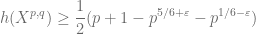
 .
. . Giving us for each
  as q runs through primes larger than
  is a
is a  -regular one for each prime
  and if the quadratic reciprocity
  then
then  . This is what I am going to do in this post.
 be the set of quaternions with
  coefficient, i.e.


 is the usual
  .
. consists of points with only odd first coordinate or points lying on spheres of radius
  and having only even first coordinate. One can easily check
  on
on  if there exists
  s.t.
s.t.  .
. , let
, let  be the quotient map.
 ,
,  carries an induced multiplication with unit.
 has exactly
  integer solutions. Hence the sphere of radius
  -tuple
  exactly one is of a different parity from the rest, depending on whether
  or
or  . Restricting to solutions where the first coordinate is non-negative, having different parity from the rest (in case the first coordinate is
  to be canonical), this way we obtain exactly
  solutions.
 be this set of
  s represent the solutions where the first coordinate is exactly
  generates
  and
and  . By definition
  and
and  is injective on
  .
. , this is a
  generares
  a non-trivial cycle.
  . Since
  is a Cayley graph, we may assume
  .
. , for some
  .
. for all
  , the word
  cannot contain either
  or
or  , hence cannot be further reduced.
 in
in  we have
 .
. must have a unique factorization
  where
where  is a reduces word of length
  .
. mod
mod 
 .
. ,
,  is a central subgroup.
 ,
,  . Which means we have well defined homomorphism
 .
. , if
, if  we have
  is injective on
  .
. .
. generates
  . Hence
  be a cycle in
  such that
  for
for  .
. ,
,  . Note that from the above arguement we know
  . In particular, this implies
  cannot all be
  .
. ,
,  hence
hence 
 hence
hence  for all cycle. i.e.
  .
. , i.e.
  .
. , we have
  is even. Let
  .
. , we also have
 .
. ,
,  .
. we will have
  . Then
  .
. must be divisible by
  , hence
  ,
,  , hence
  . Contradiction.
 .
.
 is the collection of all differentiable curves
  of the tangent bundle (depending continuously on the base point). We may attempt to define the metric
 is the collection of curves connecting
  for all
  . (i.e. we are only allowed to go along directions in the sub-bundle.
 -plane at all points. It’s easy to realize that now we are ‘stuck’ in the same height: any two points with different
  coordinate will have no curve connecting them (hence the distance is infinite). The resulting metric space is real number many discrete copies of
  away from the original point
  going along
  real entry Heisenberg group
  (all
(all 
 .
. (tangent space of the identity element), the elements
  and
and  form a basis.
 of the tangent bundle generated by infinitesimal left translations by
  . Since the metric
  for each
  .
. and
and  .
.
 ,
, -direction stay the same, i.e. a bunch of horizontal lines connecting the original
  planes orthogonally.
 -direction but also adds a height
 to
to  . –since going along the
 in fact up to a constant going along such loop gives the actual distance.
 ?
? in
in  . This gives
  .
. :
:
 . (A lot shorter compare to length
  , it’s much more efficient to travel in the C-C metric.
 (meaning bounded from both inside and outside with a constant factor). Hence the volume of balls grow like
  .
.
