Longest shortest geodesic on a 2-sphere

October 31, 2011November 1, 2011 ConanLeave a comment

This is a little note about constructing a Riemannian 2-sphere which has longer shortest geodesic than the round 2-sphere of same area.

—– Background Story —–

So there has been this thing called ‘mathematical conversations’ at the IAS, which involves someone present a topic that’s elementary enough to be accessible to mathematicians in all fields and yet can be expanded in different directions and lead into interesting interdisciplinary discussions.

Nancy Hingston gave one of those conversations about simple geodesics on the two-sphere one night and I was (thanks to Maria Trnkova who dragged me in) able to attend.

So she talked about some fascinating history of proving the existence of closed geodesics and later simple closed geodesics on generic Riemannian two-spheres.

Something about this talk obviously touched my ‘systolic nerve’, so when the discussion session came up I asked whether we have bounds on ‘length of longest possible shortest closed geodesic on a sphere with unit area’. The question seem to have generated some interest in the audience and resulted in a back-and-forth discussion (some of which I had no clue what they were talking about). So the conclusion was at least nobody knows such a result on top of their head and perhaps optimum is obtained by the round sphere.

—– End of Story —-

A couple of post-docs caught me afterwards (Unfortunately I didn’t get their names down, if you happen to know who they are, tell me~) and suggested that suspending a smooth triangular region and smoothen the corners might have longer shortest geodesic than the round sphere:

The evidence being the fact that on the plane a rounded corner triangular contour has larger ‘width’ than the disc of same area. (note such thing can be made to have same width in all directions)

Well that’s pretty nice, so I went home and did a little high-school computations. The difficulty about the pillow is that the shortest geodesic isn’t necessarily the one that goes through the ‘tip’ and ‘mid-point of the base’, something else might be shorter. I have no idea how to argue that.

A suspicious short geodesic:

So I ended up going with something much simpler, namely gluing together two identical copies of the flat equilateral triangles. This can be made to a Riemannian metric by smoothing the edge and corners a little bit:

Okay, now the situation is super simple~ I want to prove that this ‘sphere’ (let’s call it $S$ from now on) has shortest geodesic longer than the round sphere ( $\mathbb{S}^2$ )!

Of course we suppose both $S$ and $\mathbb{S}^2$ has area 1.

Claim: The shortest geodesic on $S$ has length $\sqrt[4]{12}$ (which is length of the one through the tip and mid-point of the opposite edge.)

Proof: The shortest closed geodesic passing through the corner is the one described above, since any other such geodesics must contain two symmetric segments from the corner to the bottom edge on the two triangles, those two segments alone is longer than the one orthogonal to the edge.

That middle one has length $2h$ where

$A(\Delta) = 1/2 = h^2/\sqrt{3}$

i.e. $h = \sqrt[4]{3} / \sqrt{2}, \ \ell = 2h = \sqrt[4]{12}$

The good thing about working with flat triangles is that now I know what the closed geodesics are~

First we observe any closed geodesic not passing through the corner is a periodical billiard path in the triangular table with even period.

So let’s ‘unfold’ the triangles on the plane. Such periodic orbits correspond to connecting two corresponding points on a pair of identified parallel edges and the segment between them intersecting an even number of tiles.

W.L.O.G we assume the first point in on edge $e$ . Since we are interested in orbits having shortest length, let’s take neighborhood of radius $\sqrt[4]{12} + \epsilon$ around our edge $e$ : (all edges with arrows are identified copies of $e$ )

There are only 6 parallel copies of $e$ in the neighborhood:

Note that no matter what point $p$ on $e$ we start with, the distance from $p$ to another copy of it on any of the six edges is EQUAL to $\sqrt[4]{12}$ . (easy to see since one can slide the segments to begin and end on vertices.)

Hence we conclude there are no shorter periodic billiard paths, i.e. the shortest closed geodesic on $S$ has length $\sqrt[4]{12}$ .

Note it’s curious that there are a huge amount of closed geodesics of that particular length, most of them are not even simple! However it seems that after we smoothen $S$ to a Riemannian metric, the non-simple ones all become a little longer than that simple one through the corner. I wonder if it’s possible that on a Riemannian sphere the shortest closed geodesic is a non-simple one.

Anyways, now let’s return to $\mathbb{S}^2$ ~ So the surface area is $1$ hence the radius is $r= \sqrt{1/4\pi} = \frac{1}{2\sqrt{\pi}}$

Any closed geodesics is a multiple of a great circle, hence the shortest geodesic has length $2 \pi r = \sqrt{\pi}$ , which is just slightly shorter than $\sqrt[4]{12} \approx \sqrt{3.4}$ .

Now the natural question arises: if the round sphere is not optimum, then what is the optimum?

At this point I looked into the literature a little bit, turns out this problem is quite well-studied and there is a conjecture by Christopher Croke that the optimum is exactly $\sqrt[4]{12}$ . (Of course this optimum is achieved by our singular triangle metric hence after smoothing it would be $< \sqrt[4]{12}$ .

There is even some recent progress made by Alex Nabutovsky and Regina Rotman from (our!) University of Toronto! See this and this. In particular, one of the things they proved was that the shortest geodesic on a unit area sphere cannot be longer than $8$ , which I believe is the best known bound to date. (i.e. there is still some room to $\sqrt[4]{12}$ .)

Random remark: The essential difference between this and the systolic questions is that the sphere is simply connected. So the usual starting point, namely ‘lift to universal cover’ for attacking systolic questions does not work. There is also the essential difference where, for example, the question I addressed above regarding whether the shortest geodesic is simple would not exist in systolic situation since we can always split the curve into two pieces and tighten them up, at least one would still be homotopically non-trivial. In conclusion since this question sees no topology but only the geometry of the metric, I find it interesting in its own way.

On Uryson widths

February 21, 2011February 21, 2011 ConanLeave a comment

This is a note on parts of Gromov’s paper ‘width and related invariants of Riemannian manifolds’ (1988).

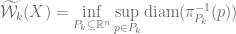
For a compact subset $C$ of $\mathbb{R}^n$ , we define the k-codimensional width (or simply k-width) to be the smallest possible number $w$ where there exists a k-dimensional affine subspace $P_k \subseteq \mathbb{R}^n$ s.t. all points of $C$ is no more than $w$ away from $P_k$ .

i.e.

$\displaystyle{W}_k(C) = \inf_{P_k \subseteq \mathbb{R}^n} \sup_{p\in C} \mbox{dist}(p, P_k)$
where $\mbox{dist}(p, P_k)$ is the length of the orthogonal segment from $p$ to $P_k$ .

It’s easy to see that, for any $C$ ,

$\mathcal{W}_0(C) \geq \mathcal{W}_1(C) \geq \cdots \geq \mathcal{W}_n(C) = 0$ .

At the first glance it may seems that $\mathcal{W}_0(C) = \frac{\mbox{diam}(C)}{2}$ . However it is not the case since for example the equilateral triangle of side length $1$ in $\mathbb{R}^2$ has diameter $1$ but 0-width $\frac{1}{\sqrt{3}}$ . In fact, by a theorem of Jung, this is indeed the optimum case, i.e. we have:

$\frac{1}{2}\mbox{diam}(C) \leq \mathcal{W}_0(C) \leq \sqrt{\frac{n}{2(n+1)}}\mbox{diam}(C)$

At this point one might wonder (at least I did), if we want to invent a notion that captures the ‘diameter’ after we ‘forget the longest k-dimensions’, a more direct way seem to be taking the smallest possible number $w'$ where there is an orthogonal projection of $C$ onto a $k$ dimensional subspace $P_k$ where any point $p \in P_k$ has pre-image with diameter $\leq w'$ .

i.e.

$\displaystyle \widetilde{\mathcal{W}_k}(X) = \inf_{P_k \subseteq \mathbb{R}^n} \sup_{p \in P_k} \mbox{diam}(\pi^{-1}_{P_k}(p))$

Now we easily have $\mbox{diam}(C) = \widetilde{\mathcal{W}_0}(C) \geq \widetilde{\mathcal{W}_1}(C) \geq \cdots \geq \widetilde{\mathcal{W}_n}(C) = 0$ .

However, the disadvantage of this notion is, for example, there is no reason for a semicircle arc to have 1-width 0 but a three-quarters circular arc having positive 1-width.

Since we are measuring how far is the set from being linear, taking convex hull should not make the set ‘wider’ $\widetilde{\mathcal{W}_k}$ , unlike $\widetilde{\mathcal{W}_k}$ is not invariant under taking convex hulls. Note that for convex sets we do have

$\frac{1}{2}\widetilde{\mathcal{W}_k}(C) \leq \mathcal{W}_k(C) \leq \sqrt{\frac{n-k}{2(n-k+1)}}\widetilde{\mathcal{W}_k}(C)$

$\mathcal{W}_k(C) = 0$ iff $C$ is contained in a $k$ -plane.

We now generalize this notion to general metric spaces:

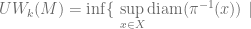
Definition: The Uryson k-width of a compact metric space $M$ is the smallest number $w$ where there exists $k$ dimensional topological space $X$ and a continuous map $\pi: M \rightarrow X$ where any point $x \in X$ has pre-image with diameter $\leq w$ .

i.e. $\displaystyle UW_k(M) = \inf \{ \ \sup_{x \in X} \mbox{diam}(\pi^{-1}(x)) \ |$

$\dim{X} = k, \pi:M \rightarrow X \ \mbox{is continuous} \}$

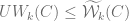Note: Here dimension is the usual covering dimension for topological spaces: i.e. a topological space $X$ is $n$ dimensional if any finite cover of $X$ has a finite refinement s.t. no point of $X$ is contained in more than $n_1$ sets in the cover and $n$ is the smallest number with this property.

For compact subsets $C$ of $\mathbb{R}^n$ with induced metric, we obviously we have $UW_k(C) \leq \widetilde{\mathcal{W}_k}(C)$ since the pair $(P_k, \pi_{p_k})$ is clearly among the pairs we are minimizing over.

Speaking of topological dimensions, one of the classical results is the following:

Lebesgue’s lemma: Let $M=[0,1]^n$ be the solid n-dimensional cube, then for any topological space $X$ with $\dim(X)<n$ and any continuous map $p: M \rightarrow X$ , we have image of at least one pair of opposite $(n-1)$ -faces intersect.

Since the conclusion is purely topological, this applies equally well to rectangles. i.e. for $M = [0, L_1] \times [0, L_2] \times \cdots \times [0, L_n]$ , $L_1 \geq L_2 \geq \cdots \geq L_n$ , we have $UW_{n-1}(M) \geq L_n$ ; furthermore, $UW_k(M) \geq L_{k+1}$ for all $k$ .

(If the later statement does not hold, we write $M$ as $M_1 \times M_2$ , $M_1$ being the product of the first $(k+1)$ coordinates. Now $UW_k(M) \geq UW_k(M_1) \geq L_{k+1}$ ).

In light of the earlier post about minimax inequality, we should note that if we restrict $X$ to be a homeomorphic copy of $\mathbb{R}^k$ then the notion is the same as the minimax length of fibres. In particular as proved in the post the minimax length of the unit disc to $\mathbb{R}$ is 2.

Exercise: Check that for the unit $2$ -disk, $UW_1(D^2) = \sqrt{3}$ , i.e. the optimum is obtained by contracting the disc onto a triod.

Hence it can indeed be strictly smaller than merely taking $\mathbb{R}^k$ as the targeting space, even for simply connected sets. This gives a better measurement of ‘width’ in the sense that, for example, the $\varepsilon$ neighborhood of a tree will have $1-width$ about $2 \varepsilon$ .

Intergal geometry and the minimax inequality in a nutshell

February 7, 2011February 7, 2011 Conan1 Comment

The goal for most of the posts in this blog has been to take out some very simple parts of certain papers/subjects and “blow them up” to a point where anybody (myself included) can understand. Ideally the simple parts should give some inspirations and ideas towards the more general subject. This one is on the same vein. This one is based on parts of professor Guth’s minimax paper.

In an earlier post, we talked about the extremal length where one is able to bound the “largest possible minimum length” (i.e. the “maximum minimum length“) of a family of rectifiable curves under conformal transformation. When combined with the uniformization theorem in for surfaces, this becomes a powerful tool for understanding arbitrary Riemannian metrics (and for conformal classes of metrics in higher dimensions).

However, in ‘real life’ we often find what we really want to bound is, instead, the “minimum maximum length” of a family of curves, for example:

Question: Let $\mathbb{D} \subseteq \mathbb{R}^2$ be the unit disc. Given any family $\mathcal{F}$ of arcs with endpoints on $\partial \ \mathbb{D}$ and $\mathcal{F}$ foliates $\mathbb{D}$ , then how short can the logest arc in $\mathcal{F}$ possibly be?

In other words, let $\mathbb{F}$ be the collection of all possible such foliations $\mathcal{F}$ as above, what is

$\displaystyle \inf_{\mathcal{F} \in \mathbb{F}} \ \sup_{A \in \mathcal{F}} \ \ell(A)$ ?

After playing around a little bit with those foliations, we should expect one of the fibres to be at least as long as the diameter ( i.e. no foliation has smaller maximum length leaf than foliating by straight lines ). Hence we should have

$\displaystyle \inf_{\mathcal{F} \in \mathbb{F}} \ \sup_{A \in \mathcal{F}} \ \ell(A) = 2$ .

This is indeed easy to prove:

Proof: Consider the map $f: S^1 \rightarrow S^1$ where $S^1 = \partial \ \mathbb{D}$ , $f$ switches the end-points of each arc in $\mathcal{F}$ . It is easy to check that $f$ is a continuous, orientation reversing homeomorphism of the circle (conjugate to a reflection). Let $p, q$ be its fixed points, $L_1, L_2$ be the two arcs in $S^1$ connecting $p$ to $q$ .

Let

$g: z \mapsto -z$

be the antipodal map on $S^1$ .

Suppose $p \neq g(q)$ then one of $L_1, L_2$ is longer than $\pi$ , say it’s $L_1$ .

Then we have

$f \circ g (L_1) \subseteq L_1$ .

Hence $f \circ g$ has a fixed point $m$ in $L_1$ , i.e. $f(m) = -m$ .

There is a fibre $A$ in $\mathcal{F}$ with endpoints $m, -m$ , the fibre must have length

$\ell(A) \geq d(-m,m) = 2$ .

The remaining case is trivial: if $p = g(q)$ then both $L_1$ and $L_2$ gets mapped into themselves orientation-reversingly, hence fixed points still exists.

Establishes the claim.

Instead of the disc, we may look at circles that sweep out the sphere (hence to avoid the end-point complications):

Theorem: Any one-parameter family of circles that foliates $S^2$ (except two points) must have the largest circle being longer than the equator.

This is merely applying the same argument, i.e. one of the circles needs to contain a pair of antipodal points hence must be longer than the equator.

In order for easier generalization to higher dimensions, with slight modifications, this can be formulated as:

Theorem: For any $f: T^2 \rightarrow S^2$ having non-zero degree, there is $\theta \in S^1$ where $\ell(f(S^1 \times \{ \theta \})$ is larger than the equator.

Hence in higher dimensions we can try to prove the same statement for largest image of a lever $k$ -sphere under $f: S^k \times S^{n-k} \rightarrow S^n$ . However before we do that I would like to highlight some intergal geometry machineries that are new to me but seemingly constantly used in proving those kinds of estimates. We shall get some idea of the method by showing:

Theorem: Let $\mathbb{R}P^n$ be equipped with the round metric. $p^k \subseteq \mathbb{R}P^n$ be a ‘flat’ $k$ -dimensional plane. Then any $k$ -chain $z^k \subseteq \mathbb{R}P^n$ in the same $k$ dimensional homology class as $p^k$ must have volume at least as large as $p^k$ .

Proof: Let $Gr(\mathbb{R}P^n, n-k)$ be the set of all $(n-k)$ -planes in $\mathbb{R}P^n$ (i.e. the Grassmannian).

There is a standard way to associate a measure $\mu$ on $Gr(\mathbb{R}P^n, n-k)$ :

Let $\lambda$ be the Haar measure on $SO(n+1)$ , fix some $Q \in Gr(\mathbb{R}P^n, n-k)$ .

Since $SO(n+1)$ acts on $\mathbb{R}P^n$ , for open set $S \subseteq Gr(\mathbb{R}P^n, n-k)$ , we set

$\mu(S) = \lambda( \{ T \in SO(n+1) \ | \ T(Q) \in S \})$ .

–The measure of a collection of planes is the measure of linear transformations that takes the given plane to an element of the set.

Now we are able to integrate over all $(n-k)$ -planes!

For almost all $Q \in Gr(\mathbb{R}P^n, n-k)$ , since $P$ is $k$ -plane, we have $| Q \cap P | = 1$ . ( not $1$ only when they are ‘parallel’ )

Since $[z] = [p]$ in $H_k(\mathbb{R}P^n, \mathbb{Z}_2)$ , for almost all $Q$ , $z$ intersects $Q$ at least as much as $P$ does. We conclude that for almost all $Q, \ | z \cap Q | \geq 1$ .

Fact: There exists constant $C$ such that for any $k$ -chain $\Sigma^k \in \mathbb{R}P^N$ ,

$\mbox{Vol}_k(\Sigma^k) = \mathbb{E}(|\Sigma \cap Q |)$ .

The fact is obtained by diving the chain into fine cubes, observe that both volume and expectation are additive and translation invariant. Therefore we only need to show this for infinitesimal cubes (or balls) near $0$ . We won’t work out the details here.

Hence in our case, since for almost all $Q$ we have $| z \cap Q | \geq 1$ , the expectation $\mathbb{E}(|z \cap Q |) \geq 1$ .

We therefore deduce

$\mbox{Vol}_k(z) = \mathbb{E}(|z \cap Q |) \geq 1$ .

Establishes the theorem.

Remark: I found this intergal geometry method used here being very handy: in the old days I always try to give lower bounds on volume of stuff by intersecting it with planes and then pretend the ‘stuff’ were orthogonal to the plane, which is the worst case in terms of having small volume. An example of such bound can be found in the knot distorsion post where in order to lower bound the length we look at its intersection number with a family of parallel planes and then integrate the intersection.

This is like looking from one particular direction and record how many times did a curve go through each height, of course one would never get the exact length if we know the curve already. What if we are allowed to look from all directions?

I always wondered if we know the intersection number with not only a set of parallel planes but planes in all directions, then are there anything we can do to better bound the volume? Here I found the perfect answer to my question: by integrating over the Grassmannian, we are able to get the exact volume from how much it intersect each plane!

We get some systolic estimates as direct corollaries of the above theorem, for example:

Corollary: $\mbox{Sys}_1(\mathbb{R}P^2) = \sqrt{\pi/2}$ where $\mathbb{R}P^2$ carries the round metric with total volume $1$ .

Back to our minimax problems, we state the higher dimensional version:

Wish: For any $C^1$ map $f: S^k \times S^{n-k} \rightarrow S^n$ where $S^n$ carries the standard round metric, there exists some $\theta \in S^{n-k}$ with

$\mbox{Vol}_k(f(S^k\times \{\theta\})) \geq \mbox{Vol}_k(E^k)$

where $E^k \subseteq S^n$ is the $k$ -dimensional equator.

But what we have is that there is a (small) positive constant $c(n,k)$ s.t. $\mbox{deg}(f) \neq 0$ implies

$\displaystyle \sup_{\theta \in S^{n-k}} \mbox{Vol}_k(f(S^k \times \{\theta\})) \geq c(n,k) \mbox{Vol}_k(E^k)$

(shown by an inductive application of the isomperimetric inequality on $S^N$ , which is obtained from applying intergal geometry methods)

Cutting the Knot

December 13, 2010December 14, 2010 Conan10 Comments

Recently I came across a paper by John Pardon – a senior undergrad here at Princeton; in which he answered a question by Gromov regarding “knot distortion”. I found the paper being pretty cool, hence I wish to highlight the ideas here and perhaps give a more pictorial exposition.

This version is a bit different from one in the paper and is the improved version he had after taking some suggestions from professor Gabai. (and the bound was improved to a linear one)

Definition: Given a rectifiable Jordan curve $\gamma: S^1 \rightarrow \mathbb{R}^3$ , the distortion of $\gamma$ is defined as

$\displaystyle \mbox{dist}(\gamma) = \sup_{t,s \in S^1} \frac{d_{S^1}(s,t)}{d_{\mathbb{R}^3}(\gamma(s), \gamma(t))}$ .

i.e. the maximum ratio between distance on the curve and the distance after embedding. Indeed one should think of this as measuring how much the embedding ‘distort’ the metric.

Given knot $\kappa$ , define the distortion of $\kappa$ to be the infimum of distortion over all possible embedding of $\gamma$ :

$\mbox{dist}(\kappa) = \inf\{ \mbox{dist}(\gamma) \ | \ \gamma \ \mbox{is an embedding of} \ \kappa \ \mbox{in} \ \mathbb{R}^3 \}$

It was (somewhat surprisingly) an open problem whether there exists knots with arbitrarily large distortion.

Question: (Gromov ’83) Does there exist a sequence of knots $(\kappa_n)$ where $\lim_{n \rightarrow \infty} \mbox{dist}(\kappa_n) = \infty$ ?

Now comes the main result in the paper: (In fact he proved a more general version with knots on genus $g$ surfaces, for simplicity of notation I would focus only on torus knots)

Theorem: (Pardon) For the torus knot $T_{p,q}$ , we have

$\mbox{dist}(T_{p,q}) \geq \frac{1}{100} \min \{p,q \}$

To prove this, let’s make a few observations first:

First, fix a standard embedding of $\mathbb{T}^2$ in $\mathbb{R}^3$ (say the surface obtained by rotating the unit circle centered at $(2, 0, 0)$ around the $z$ -axis:

and we shall consider the knot that evenly warps around the standard torus the ‘standard $T_{p,q}$ knot’ (here’s what the ‘standard $T_{5,3}$ knot looks like:

By definition, an ’embedding of the knot’, is a homeomorphism $\varphi:\mathbb{R}^3 \rightarrow \mathbb{R}^3$ that carries the standard $T_{p,q}$ to the ‘distorted knot’. Hence the knot will lie on the image of the torus (perhaps badly distorted):

For the rest of the post, we denote $\varphi(T_{p,q})$ by $\kappa$ and $\varphi(\mathbb{T}^2)$ by $T^2$ , w.l.o.g. we also suppose $p<q$ .

Definition: A set $S \in T^2$ is inessential if it contains no homotopically non-trivial loop on $T^2$ .

Some important facts:

Fact 1: Any homotopically non-trivial loop on $\mathbb{T}^2$ that bounds a disc disjoint from $T^2$ intersects $T_{p,q}$ at least $p$ times. (hence the same holds for the embedded copy $(T^2, \kappa)$ ).

As an example, here’s what happens to the two generators of $\pi_1(\mathbb{T}^2)$ (they have at least $p$ and $q$ intersections with $T_{p,q}$ respectively:

From there we should expect all loops to have at least that many intersections.

Fact 2: For any curve $\gamma$ and any cylinder set $C = U \times [z_1, z_2]$ where $U$ is in the $(x,y)$ -plane, let $U_z = U \times \{z\}$ we have:

$\ell(\gamma \cap C) \geq \int_{z_1}^{z_2} | \gamma \cap U_z | dz$

i.e. The length of a curve in the cylinder set is at least the integral over $z$ -axis of the intersection number with the level-discs.

This is merely saying the curve is longer than its ‘vertical variation’:

Similarly, by considering variation in the radial direction, we also have

$\ell(\gamma \cap B(\bar{0}, R) \geq \int_0^{R} | \gamma \cap \partial B(\bar{0}, r) | dr$

Proof of the theorem

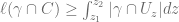
Now suppose $\mbox{dist}(T_{p,q})<\frac{1}{100}p$ , we find an embedding $(T^2, \kappa)$ with $\mbox{dist}(\kappa)<\frac{1}{100}p$ .

For any point $x \in \mathbb{R}^3$ , let

$\rho(x) = \inf \{ r \ | \ T^2 \cap (B(x, r))^c$ is inessential $\}$

i.e. one should consider $\rho(x)$ as the smallest radius around $x$ so that the whole ‘genus’ of $T^2$ lies in $B(x,\rho(x))$ .

It’s easy to see that $\rho$ is a positive Lipschitz function on $\mathbb{R}^3$ that blows up at infinity. Hence the minimum value is achieved. Pick $x_0 \in \mathbb{R}^3$ where $\rho$ is minimized.

Rescale the whole $(T^2, \kappa)$ so that $x_0$ is at the origin and $\rho(x_0) = 1$ .

Since $\mbox{dist}(\kappa) < \frac{1}{100}p$ (and note distortion is invariant under scaling), we have

$\ell(\kappa \cap B(\bar{0}, 1) < \frac{1}{100}p \times 2 = \frac{1}{50}p$

Hence by fact 2, $\int_1^{\frac{11}{10}} | \kappa \cap \partial B( \bar{0}, r)| dr \leq \ell(\kappa \cap B(\bar{0}, 1)) < \frac{1}{40}p$

i.e. There exists $R \in [1, \frac{11}{10}]$ where the intersection number is less or equal to the average. i.e. $| \kappa \cap \partial B(\bar{0}, R) | \leq \frac{1}{4}p$

We will drive a contradiction by showing there exists $x$ with $\rho(x) < 1$ .

Let $C_z = B(\bar{0},R) \cap \{z \in [-\frac{1}{10}, \frac{1}{10}] \}$ , since

$\int_{-\frac{1}{10}}^{\frac{1}{10}} | U_t \cap \kappa | dt \leq \ell(\kappa \cap B(\bar{0},1) ) < \frac{1}{50}p$

By fact 2, there exists $z_0 \in [-\frac{1}{10}, \frac{1}{10}]$ s.t. $| \kappa \cap B(\bar{0},1) \times \{z_0\} | < \frac{1}{10}p$ . As in the pervious post, we call $B(\bar{0},1) \times \{z_0\}$ a ‘neck’ and the solid upper and lower ‘hemispheres’ separated by the neck are $U_N, U_S$ .

Claim: One of $U_N^c \cap T^2, \ U_S^c \cap T^2$ is inessential.

Proof: We now construct a ‘cutting homotopy’ $h_t$ of the sphere $S^2 = \partial B(\bar{0}, R)$ :

i.e. for each $t \in [0,1), \ h_t(S^2)$ is a sphere; at $t=1$ it splits to two spheres. (the space between the upper and lower halves is only there for easier visualization)

Note that during the whole process the intersection number $h_t(S^2) \cap \kappa$ is monotonically increasing. Since 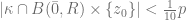$| \kappa \cap B(\bar{0},R) \times \{z_0\} | < \frac{1}{10}p$ , it increases no more than $\frac{1}{5}p$ .

Observe that under such ‘cutting homotopy’, $\mbox{ext}(S^2) \cap T^2$ is inessential then $\mbox{ext}(h_1(S^2)) \cap T^2$ is also inessential. (to ‘cut through the genus’ requires at least $p$ many intersections at some stage of the cutting process, but we have less than $\frac{p}{4}+\frac{p}{5} < \frac{p}{2}$ many interesections)

Since $h_1(S^2)$ is disconnected, the ‘genus’ can only lie in one of the spheres, we have one of $U_N^c \cap T^2, \ U_S^c \cap T^2$ is inessential. Establishes the claim.

We now apply the process again to the ‘essential’ hemisphere to find a neck in the $y$ direction, i.e.cutting the hemisphere in half in $(x,z)$ direction, then the $(y,z)$ -direction:

The last cutting homotopy has at most $\frac{p}{5} + 3 \times \frac{p}{4} < p$ many intersections, hence has inessential complement.

Hence at the end we have an approximate $\frac{1}{8}$ ball with each side having length at most $\frac{6}{5}$ , this shape certainly lies inside some ball of radius $\frac{9}{10}$ .

Let the center of the $\frac{9}{10}$ -ball be $x$ . Since the complement of the $\frac{1}{8}$ ball intersects $T^2$ in an inessential set, we have $B(x, \frac{9}{10})^c \cap T^2$ is inessential. i.e.

$\rho(x) \leq \frac{9}{10} <1$

Contradiction.

Extremal length and conformal geometry

December 6, 2010December 6, 2010 Conan2 Comments

There has been a couple of interesting talks recently here at Princeton. Somehow the term ‘extremal length’ came up in all of them. Due to my vast ignorance, I knew nothing about this before, but it sounded cool (and even somewhat systolic); hence I looked a little bit into that and would like to say a few words about it here.

One can find a rigorous exposition on extremal length in the book Quasiconformal mappings in the plane.

Let $\Omega$ be a simply connected Jordan domain in $\mathbb{C}$ . $f: \Omega \rightarrow \mathbb{R}^+$ is a conformal factor on $\Omega$ . Recall from my last post, $f$ is a Lebesgue measurable function inducing a metric on $\Omega$ where

$\mbox{Vol}_f(U) = \int_U f^2 dx dy$

and for any $\gamma: I \rightarrow \Omega$ ( $I \subseteq \mathbb{R}$ is an interval) with $||\gamma'(t)|| = \bar{1}$ , we have the length of $\gamma$ :

$l_f(\gamma) = \int_I f dt$ .

Call this metric $g_f$ on $\Omega$ and denote metric space $(\Omega, g_f)$ .

Given any set $\Gamma$ of rectifiable curves in $U$ (possibly with endpoints on $\partial U$ ), each comes with a unit speed parametrization. Consider the “ $f$ -width” of the set $\Gamma$ :

$\displaystyle w_f(\Gamma) = \inf_{\gamma \in \Gamma} l_f(\gamma)$ .

Let $\mathcal{F}$ be the set of conformal factors $f$ with $L^2$ norm $1$ (i.e. having the total volume of $\Omega$ normalized to $1$ ).

Definition: The extremal length of $\Gamma$ is given by

$\mbox{EL}(\Gamma) = \displaystyle \sup_{f \in \mathcal{F}} w_f(\Gamma)^2$

Remark: In fact I think it would be more natural to just use $w_f(\Gamma)$ instead of $w_f(\Gamma)^2$ since it’s called a “length”…but since the standard notion is to sup over all $f$ , not necessarily normalized, and having the $f$ -width squared divide by the volume of $\Omega$ , I can’t use conflicting notation. One should note that in our case it’s just the square of sup of width.

Definition:The metric $(\Omega, g_f)$ where this extremal is achieved is called an extremal metric for the family $\Gamma$ .

The most important fact about extremal length (also what makes it an interesting quantity to study) is that it’s a conformal invariant:

Theorem: Given $h: \Omega' \rightarrow \Omega$ bi-holomorphic, then for any set of normalized curves $\Gamma$ in $\Omega$ , we can define $\Gamma' = \{ h^{-1}\circ \gamma \ | \ \gamma \in \Gamma \}$ after renormalizing curves in $\Gamma'$ we have:

$\mbox{EL}(\Gamma) = \mbox{EL}(\Gamma')$

Sketch of a proof: (For simplicity we assume all curves in $\Gamma'$ are rectifiable, which is not always the case i.e. for bad maps $h$ the length might blow up when the curve approach $\partial \Omega'$ this case should be treated with more care)

This is indeed not hard to see, first we note that for any $f: \Omega \rightarrow \mathbb{R}^+$ we can define $f' : \Omega' \rightarrow \mathbb{R}^+$ by having

$f^\ast (z) = |h'(z)| (f \circ h) (z)$

It’s easy to see that $\mbox{Vol}_{f^\ast}(\Omega') = \mbox{Vol}_{f}(\Omega)$ (merely change of variables).

In the same way, $l_{f^\ast}(h^{-1}\circ \gamma) = l_f(\gamma)$ for any rectifiable curve.

Hence we have

$w_{f^\ast}(\Gamma') = w_f(\Gamma)$ .

On the other hand, we know that $\varphi: f \mapsto f^\ast$ is a bijection from $\mathcal{F}_\Omega$ to $\mathcal{F}_{\Omega'}$ , deducing

$\mbox{EL}(\Gamma) = \displaystyle ( \sup_{f \in \mathcal{F}} w_f(\Gamma))^2 = \displaystyle ( \sup_{f' \in \mathcal{F}'} w_{f'}(\Gamma'))^2 = \mbox{EL}(\Gamma')$

Establishes the claim.

One might wonder how on earth should this be applied, i.e. what kind of $\Gamma$ are useful to consider. Here we emphasis on the simple case where $\Omega$ is a rectangle (Of course I would first look at this case because of the unresolved issues from the last post :-P ):

Theorem: Let $R = (0,w) \times (0, 1/w)$ , $\Gamma$ be the set of all curves starting at a point in the left edge $\{0\} \times [0, 1/w]$ , ending on $\{1\} \times [0, 1/w]$ with finite length. Then $\mbox{EL}(\Gamma) = w^2$ and the Euclidean metric $f = \bar{1}$ is an extremal metric.

Sketch of the proof: It suffice to show that any metric $g_f$ with $\mbox{Vol}_f(R) = 1$ has at least one horizontal line segment $\gamma_y = [0,w] \times \{y\}$ with $l_f(\gamma_y) \leq w$ . (Because if so, $w_f(\Gamma) \leq w$ and we know $w_{\bar{1}}(\Gamma) = w$ for the Euclidean length)

The average length of $\gamma_y$ over $y$ is

$w \int_0^{1/w} l_f(\gamma_y) dy$

$= w \int_0^{1/w} (\int_0^w f(t, y) dt) dy = w \int_R f$

By Cauchy-Schwartz this is less than $w (\int_R f^2)^{1/2} |R|^{1/2} = w$

Since the shortest curve cannot be longer than the average curve, we have $w_f(\Gamma) \leq w$ .

Hence $\mbox{EL}(\Gamma) = \displaystyle \sup_{f \in \mathcal{F}}w_f(\Gamma)^2 = w^2$

Note it’s almost the same argument as in the proof of systolic inequality on the 2-torus.

Corollary: Rectangles with different eccentricity are not conformally equivalent (i.e. one cannot find a bi-homomorphic map between them sending each edge to an edge).

Remark: I was not aware of this a few days ago and somehow had the silly thought that there are conformal maps between any pair of rectangles while discussing with Guangbo >.< then tried to see what would those maps look like and was of course not able to do so. (there are obviously Riemann maps between the rectangles, but they don't send conners to conners, i.e. can't be extended to a conformal map on the closed rectangle).

An add-on: While I came across a paper of Odes Schramm, applying the techniques of extremal length, the following theorem seemed really cool.

Let $G = (V, E)$ be a finite planar graph with vertex set $V$ and edges $E \subseteq V^2$ . For each vertex $v$ we assign a simply connected domain $D_v$ .

Theorem: We can scale and translate each $D_v$ to $D'_v$ so that $\{ D_v \ | \ v \in V \}$ form a packing (i.e. are disjoint) and the contact graph of $D'_v$ is $G$ . (i.e. $\overline{D'_{v_1}} \cap \overline{D'_{v_2}} \neq \phi$ iff $(v_1, v_2) \in E$ .

Note: This is vastly stronger than producing a circle packing with prescribed structure.

Area777

Chasing dreams from mathematics to the real world

Tag: Systoles

Longest shortest geodesic on a 2-sphere

On Uryson widths

Intergal geometry and the minimax inequality in a nutshell

Cutting the Knot

Extremal length and conformal geometry

Share this:

Share this:

Share this:

Share this:

Share this: