(images are gradually being inserted ~)

I’m temporarily back into mathematics to (try) finish up some stuff about laminations. While I’m on this, I figured maybe sorting out some very basic (and cool) things in a little post here would be a good idea. Browsing through the blog I also realized that as a student of Dave’s I have been writing surprisingly few posts related to what we do. (Don’t worry, like all other posts in this blog, I’ll only put in stuff anyone can read and hopefully won’t be bored reading :-P)

Here we go. As mentioned in this previous post, my wonderful advisor has proved that the ending lamination space is connected and locally connected (see Gabai’08).

Definition: Let be a hyperbolic surface of genus and punctures. A (geodesic) lamination is a closed set that can be written as a disjoint union of geodesics. i.e. where each is a (not necessary closed) geodesic, is called a leaf of .

Let’s try to think of some examples:

i) One simple closed geodesic

ii) A set of disjoint simple closed geodesics

iii) A non-closed geodesic spirals onto two closed ones

iV) Closure of a single simple geodesic where transversal cross-sections are Cantor-sets

An ending lamination is a lamination where
a) the completement is a disjoint union of discs and once punctured discs (filling)
b) all leaves are dense in . (minimal)

Exercise: example i) satisfies b) and example iv) as shown satisfies both a) and b) hence is the only ending lamination.

It’s often more natural to look at measured laminations, for example as we have seen in the older post, measured laminations are natural generalizations of multi-curves and the space is homeomorphic to (Thurston) with very natural coordinate charts (given by train-tracks).

Obviously not all measured laminations are supported on ending laminations (e.g. example i) and ii) with atomic measure on the closed curves.) It is well known that if a lamination fully supports an invariant measure, then as long as the base lamination satisfies a), it automatically satisfies b) and hence is an ending lamination. This essentially follows from the fact that having a fully supported invariant measure and being not minimal implies the lamination is not connected and hence won’t be filling.

Exercise:Example iii) does not fully support invariant measures.

Scaling of the same measure won’t effect the base lamination, hence we may eliminate a dimension by quotient that out and consider the space of projective measured laminations 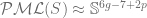. Hence we may decompose measured laminations into filling and unfilling ones. i.e.

where projects to the ending laminations via the forgetting measure map .

This decomposition of the standard sphere is mysterious and very curious in my opinion. To get a sense of this, let’s take a look at the following facts:

Fact 1: is a union of countably many disjoint hyper-discs (i.e. discs of co-dimension ).

Well, if a measured lamination is unfilling, it must contain some simple closed geodesic as a leaf (or miss some simple closed geodesic). For each such geodesic , there are two possible cases:

Case 1: is non-separating. The set of measured laminations that missed is precisely the set of projective measured laminations supported on , hence homeomorphic to we may take any such measured lamination, disjoint union with , we may assign any ratio of wrights to and the lamination. This corresponds to taking the cone of with vertex being the atomic measure on . Yields a disc of dimension .

Case 2: is separating. Similarly, the set of measured laminations missing is supported on two connected surfaces with total genus and total punctures .

To describe the set of projective measured laminations missing , we first determine the ratio of measure between two connected components and then compute the set of laminations supported in each component. i.e. it’s homeomorphic to where and and .

Exercise: check this is a sphere. hint: if , we have:

Again we cone w.r.t. the atomic measure corresponding to , get a hyper disc.

At this point you may think ‘AH! is only a countable union of hyper-discs! How complicated can it be?!’ Turns out it could be, and (unfortunately?) is, quite messy:

Fact 2: is dense in .

This is easy to see since any filling lamination is minimal, hence all leaves are dense, we may simply take a long segment of some leaf where the beginning and end point are close together on some transversal, close up the segment by adding a small arc on the transversal, we get a simple closed geodesic that’s arbitrarily close to the filling lamination in . Hence the set of simple closed curves with atomic measure are dense, obviously implying dense.

So how exactly does this decomposition look like? I found it very mysterious indeed. One way to look at this decomposition is: we know two discs can intersect if and only if their corresponding curved are disjoint. Hence in some sense the configuration captures the structure of the curve complex. Since we know the curve complex is connected, we may start from any disc, take all discs which intersect it, then take all discs intersecting one of the discs already in the set, etc.

We shall also note that all discs intersecting a given disc must pass through the point corresponding to the curve at the center. Hence the result will be some kind of fractal-ish intersecting discs:

(image)

Yet somehow it manages to ‘fill’ the whole sphere!

Hopefully I have convinced you via the above that countably many discs in a sphere can be complicated, not only in pathological examples but they appear in ‘real’ life! Anyways, with Dave’s wonderful guidance I’ve been looking into proving some stuff about this (in particular, topology of ). Hopefully the mysteries would become a little clearer over time~!