A Chinese new year greeting~

January 23, 2012March 12, 2012 Conan5 Comments

So this is the first day of the Chinese new year, classes/seminars still haven’t resumed since December 17th, still two weeks to go before anything starts…

Anyways, I’m borrowing this occasion to thank everyone for continuously supporting this blog! We’ve had a great year, check the annual report at the end of the post for details.

As some of you may already know, I have decided that mathematics is not going to be my life-long career. So far it’s not clear in which direction will this blog go, it’s simply too important to abandon. I guess only time would tell. However, expect changes.

Finally, a sketch I doodled up last night~ Happy Chinese new year!

(btw, for those who have seen me in winter, yes I’m waring that Klein bottle hat in the picture!)

The WordPress.com stats helper monkeys prepared a 2011 annual report for this blog.

Here’s an excerpt:

The concert hall at the Sydney Opera House holds 2,700 people. This blog was viewed about 15,000 times in 2011. If it were a concert at Sydney Opera House, it would take about 6 sold-out performances for that many people to see it.

Click here to see the complete report.

Sumsets, in discrete and continuous settings

December 12, 2011December 16, 2011 Conan4 Comments

In the past few years, there are 137 papers with the term ‘sumset’ in its title; and 50 more with ‘sum-set’. Ok the above statement was stolen from a talk I happen to be sitting in, by Noga Alon.

As usual, in the middle of the talk I got carried away by some ‘trivial facts’ he wrote down which are only slightly related to the main content. So I thought about that for during the rest of the talk (and also a little bit afterwards).

This time the curious point pops up when he was motivating why people should be studying chromatic number of random Cayley graphs by its application to sumsets.

Definition: In a vector space $X$ , a sumset $S \subseteq X$ is a set that can be represented as the Minkowski sum of another set with itself. i.e. $S = A+A$ where $A+A = \{ a_1+a_2 \ | \ a_1, a_2 \in A \}$ .

It was mentioned that given a large $p$ , if we look at sets in $\mathbb{Z}_p$ , then all sets with large cardinality must be sumsets.

This fact is first published by Ben Green who also raised the natural question:

Question: What’s the lower bound $M(p)$ such that all subsets $S \subseteq \mathbb{Z}_p$ with $|S| > M(p)$ must be a sumset?

Let’s first see why all sets of large cardinality must be sumsets: Well as we all know $\mathbb{Z}_p = \mathbb{Z}_p + \mathbb{Z}_p$ (can also be expressed as many other sums) is a sumset. Hence the first non-trivial case is $\mathbb{Z}_p \backslash \{x\}$ :

The way I think of sumsets is that they are projections of product sets in the angle $3/4 \pi$ :

Hence our goal is to make up a set $S_x$ such that the projection, after mod $p$ , is everything except for the point $x$ . Well, this isn’t too hard, first note the image of the ‘interval’ $\{ x+1, x+2, \cdots, p+x-1 \}$ after mod $p$ is exactly the set we wanted. Now we just need to make $A \times A$ project to the interval! $A = \{ x/2 +1, x/2 + 2, \cdots (p+x)/2 -1 \}$ will do. (Here by $C/2$ we meant that it’s the integer $C/2$ when $C$ is even and $(C+p)/2$ when it’s odd.

Note that since $x \in \mathbb{Z}_p$ , $A + A$ is actually a square in $\{ 0, 1, \cdots, p-1 \}^2$ and only “warped” in mod $p$ after we project it to $\{ 0, 1, \cdots, 2p-2 \}$ .

So we just showed all sets with one missing element is a sumset~ Now let’s move to sets of size $p-2$ …(Don’t worry, I’m not going on to 3 and the length of this post will be finite :-P)

In contrast to the above argument which actually works in the continuous setting and shows the Lie group $S^1$ missing any interval is a sumset, this time we actually need to use the fact that our space is discrete and finite.

Note first that the property of being a sumset is invariant under scaling and translating by an integer. Indeed,

$n\cdot S = \{ ns \ | \ s \in S \}$

$= \{n(a_1+a_2) \ | \ a_1, a_2 \in A\} = n \cdot A + n \cdot A$

and of course $S+t = (A+t/2) + (A+t/2)$ .

Now no matter which two points $a,b$ we delete, i.e. $S = \mathbb{Z}_p \backslash \{a, b \}$ , we may let $S' = (b-a)^{-1} \cdot (S-a)$ . We have $S' = \mathbb{Z}_p \backslash \{0, 1\}$ , which is the projection of the square $I^2 = \{ 1,2, \cdots, (p-1)/2 \}^2$ .

Hence $S = [(b-a) \cdot I + a/2] + [(b-a) \cdot I + a/2]$ is a sumset.

After playing around with the torus for a little bit, I believe in the continue case we can still write $S^1$ deleting two (small) intervals as a sumset $A+A$ where $A$ is a union of no more than 4 intervals. There are quite a few cases involved concerning the spacing between small intervals, hence I’ll just draw an example:

(By the way, this is about as far as I got daydreaming during the lecture, the rest came from the sources I looked up afterwards.)

Unfortunately since the scaling and translating gived only two degrees of freedom, the above argument fails when considering sets missing three points. (Playing with torus as I first tried, however, might still work)

Back to our question, so now we know at least $M_p < p-2$ the natural thing to study is of course how does it grow with $p$ . Recall that we denoted $M_p = p - f(p)$ , hence the problem is equivalent to giving asymptotic lower bounds for $f(p)$ .

So this is quite curious, what do you think? Is $f(p)$ just a counstant? (such as $2$ , or $3$ ?) Or is it always more than a fixed proportion of $\mathbb{Z}_p$ ? (say any set containing 99% of the elements must be a sumset?) Or something in-between?

As one might have expected, $f(p)$ is more than a constant,

Theorem: (Green) $f(p) \geq \frac{1}{9} \log_2(p)$ .

It’s also not as large as a fixed percentage:

Theorem: (Gowers-Green) $f(p) \leq C \cdot p^2/3 \log(p)$

So it’s something ‘in-between’. Interesting…So what is this number? This is an open question in general, by applying methods of Cayley graphs and their spectrums, the speaker (of the talk) was able to improve the above bounds (in this other paper):

Theorem: (Alon) $c \cdot \sqrt{\frac{p}{\log{p}}} \leq f(p) \leq C \cdot \frac{ p^2/3}{ \log(p)^{1/3}}$

However one should expect that

Conjecture: (Green) $f(p) \sim p^{1/2+O(1)}$ .

Having knowing absolutely nothing about the subject (or combinatorics in general), my first reaction about this is that perhaps, if we look at $\mathbb{Z}_p$ where $p$ is roughly $N^2$ , let $S$ be the set missing $N$ equally spaced points, now if we want to write $S$ as a sumset that’s like finding a product $A \times A \subseteq \mathbb{T}^2$ that misses all $N$ diagonal circles and have at least $N$ points in each thin strip to ‘block’ every diagonal circle in the strip.

I think this set looks (by the same philosophy as when we play around with the two intervals on the tori case) fairly hard to express as a sum. i.e. when we are exactly in $\mathbb{Z}_{N^2}$ , we can probably ‘just’ do it by choosing one representative from each mod $N$ class and place them in the $N$ strips. But looks as if the ‘resolution’ is any lower, (i.e. $p$ is a little smaller and we still have about $N$ equally spaced holes), we would not have enough freedom to place the points.

Anyways, that last remark might be completely nonsense~ The conjecture is interesting, tho.

The Schwartz lantern

November 28, 2011November 29, 2011 Conan5 Comments

It’s thanksgiving, let’s have some fun in lantern-making!

This thing called Schwartz lantern initially came up in a talk some years ago, I vaguely remembered it as ‘a cool example where the refining triangle approximation of a smooth surface fail to converge in area’. Anyways, it came up again recently as I was talking to some German postdoc working in ‘discrete differential geometry’. As the example was mentioned, he took a napkin and started folding…and I just realized this lantern can actually be made with a piece of flat paper!

Given a compact, smooth surface (possibly with boundary) embedded in $\mathbb{R}^3$ , we can approximate it by a PL surface with all vertices on the surface and having only triangular faces. (just like what’s done in many computer graphic softwares nowadays).

Question: When the vertices of the faces gets denser and denser and the diameter of triangles converge to $0$ , does the area of the PL surface converge to the area of the surface?

Ok, to explain why I found this being a quite curious little question, let’s prove a couple of trivial observations:

Trivial fact #1: The sequence of PL surfaces as described above does Hausdorff converge to the smooth surface.

Proof:Since our surface is smooth, as the diameter of the triangles converge to $0$ , the length of the geodesic between two vertices is roughly the length of the edge in the 1-skeleton of the PL surface. In particular, less than twice its length.

Now by compactness we have a positive injectivity radius, implying that for small enough length $c$ , the diameter (on the surface) of region enclosed by any loop of length most $c$ is controlled by $c$ (say it’s $\leq f(c)$ which converge to $0$ as $c \rightarrow 0$ ). Now the $\mathbb{R}^3$ diameter of the region is of course even smaller than its surface diameter.

In conclusion, when all triangles have small diameter $\varepsilon$ (hence all its sides have length at most $\varepsilon$ ), the geodesic triangle on the surface has parameter less than $6 \varepsilon$ . So $\mathbb{R}^3$ diameter of the geodesic triangle is no more than $f(6 \varepsilon)$ . Hence the surface is contained in the $f(6\varepsilon)$ -neighbourhood of the vertex set.

Obviously the PL surface is also contained in this neighbourhood. Hence the Hausdorff distance is at most $f(6\varepsilon)$ , which converges to $0$ .

Trivial fact #2: For curves in $\mathbb{R}^2$ (in fact, or $\mathbb{R}^n$ ), the length converges.

Proof: Well…what can I say…see any undergrad calculus book? (well, all we need is that smooth curves are rectifiable. Of course they are…

So from the above observations, does it kinda smell like the area would converge? (If you know the answer, you should pretend you don’t and nod at this point :-P) Well, the fact is they don’t have to converge! (otherwise why are we making counter-examples here?) Furthermore, this is first discovered by a super-cool dude – Schwartz! He even wrote a paper about it back in 1880.

How can this be possible? You might have already observed that with some simple curvature bounding, we can push the argument for trivial fact #1 to show that area of the curved surface is controlled above by the straight surface, The point being (perhaps to one’s surprise) that the ‘straight surface’ can be a lot LARGER than the curved one!

So the example is a sequence of ‘lanterns’ converging to a standard cylinder (say of height and circumference both equal to $1$ ), i.e. PL surfaces with triangular faces, vertices on the cylinder, with smaller and smaller ‘grids’, and the sum of areas of the triangle blows up to infinity.

As shown above, if we have put $N^4$ points on the cylinder, $N$ points along the circumference and $N^3$ in the vertical direction (picture is not to scale); connected to form triangles in the above way.

Now all triangles are isosceles and identical. Doing some middle-school geometry shows that they have base length $\geq \frac{1}{2N}$ and height 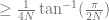$\geq \frac{1}{4N}\tan^{-1}(\frac{\pi}{2N})$ (this calculates the distance between the midpoint of the base to the cylinder surface).

Having $2N^4$ triangles means the area $A_N$ of the PL surface is at least $N^4 \times \frac{1}{2N} \times \frac{1}{4N}\tan^{-1}(\frac{\pi}{2N})$ when $N$ large, $\tan^{-1}(\frac{\pi}{2N}) \sim \frac{\pi}{2N} \geq \frac{1}{N}$ . Hence the $A_N \geq \frac{N}{8}$ blows up to infinity.

Is this pretty cool? This lantern also have an interesting feature that, if we define ‘curvature’ on vertices to be the sum of angles attached to that vertex, (and of course the curvature on the edge between two flat faces shall be $0$ ), then all lanterns have curvature $0$ everywhere, just as in the smooth cylinder! i.e. it can be made by folding a single piece of flat paper.

Let’s note that although the triangles are getting uniformly smaller, they do become ‘thinner and thinner’ in the example. In fact this is the only way it can go wrong, i.e. it can be shown that if we further require the triangles to have bounded eccentricity then the area does converge.

Add-on: I actually made the lantern! They are interesting to fold, aesthetically pleasing and even functional! (you’ll see light flaring out in an interesting way)

Trying it out while one thinks about problems is highly amusing and recommended~

All one needs to do is:

Tips on folding:

1. Be sure to make all diagonal lines positive fold and horizontal lines negative.

2. Make the diagonals cross an even number of horizontals or else after you finish all diagonals, you’ll end up with left and right-facing diagonals not crossing on the horizontal (i.e. you’ll need to double the number of horizontals to make it work again)

3. After finishing all lines, it might be hard at first to make the whole thing ‘fold up’. The trick being to make sure all ‘crosses’ are ‘poped-out’ on the whole surface. The final folding process does not work locally!

4. Although theoretically you can take an arbitrarily long strip of paper with unit width to make unit-sized lantern, but in order to not make a million folds and have super-sharp angles between the diagonal and horizontal; I recommend not being too aggressive on the length :-P (square-ish papers are good enough)

Have fun!~

A not-very-good picture of my lantern (larking light bulb…>.<)

Haken manifolds and virtual Haken conjecture

November 21, 2011November 22, 2011 Conan1 Comment

Hi people~ My weekends have been unfortunately filled up with grading undergrad assignments for the last couple of weeks >.< I'll try to catch up on blogging by finding some other time slot during the week.

As a grand-student of Thurston's I feel obligated to end my ignorance regarding Haken manifolds. I guess it's a good idea to start by writing my usual kids-friendly exposition here.

In the rest of the post, $M$ is a compact (so perhaps with boundary), orientable, irreducible (meaning each embedded 2-sphere bounds a ball) 3-manifold.

Definition: A properly embedded oriented surface $S \subseteq M$ is incompressible if $S$ is not the 2-sphere and any simple closed curve on $S$ which bounds an embedded disc in $M \backslash S$ also bounds one in $S$ .

Figure 1

In other words, together with Dehn’s lemma this says the map $\varphi: \pi_1(S) \rightarrow \pi_1 (M)$ induced by the inclusion map is injective.

Note that the surface $S$ could have boundary, for example:

Figure 2

Definition: $M$ is Haken if it contains an incompressible surface.

Okay, at this point you should be asking, what’s good about Haken manifolds? The beauty about it is that, roughly speaking, once you find one incompressible surface in the manifold, you can just keep finding them until the manifold is completely chopped up into balls by incompressible surfaces.

Theorem: (Haken) Any Haken 3-manifold $M$ contains a hierarchy $S_0 \subseteq S_1 \subseteq \cdots \subseteq S_n$ where

1. $S_0$ is an incompressible surface in $M$
2. $S_i = S_{i-1} \cup S$ where $S$ is an incompressible surface for the closure of some connected component $K$ of $latex $M \backslash S_{i-1}$
3. $M \backslash S_n$ is a union of 3-balls

Sketch of proof: This is much simpler than it might appear to be. The point is (at least in my opinion), except for trivial cases as long as a manifold has boundary it must be Haken.

Lemma: If $\partial M$ has a component that’s not $\mathbb{S}^2$ then $M$ is Haken.

The proof of the lemma is merely that any such $M$ will have infinite $H_2$ hence by the sphere theorem it will contain an embedded surface with non-trivial homology, if such surface is compressible then we just cut along the boundary of the compressing disc and glue two copies of it. This does not change the homology. Hence at the end we will arrive at a non-trivial incompressible surface.

Figure 3

Now back to proving of the theorem, so we start by setting $S_0$ to be an incompressible surface given by $M$ being Haken.

Now since $M$ is irreducible, we cut along $S_0$ , i.e. take the closure of each component (may have either one or two components) of $M\backslash S_0$ . Those will have a non-spherical boundary component, hence by lemma containing homologically non-trivial incompressible surface.

This process continuous as long as some pieces has non-spherical boundary components. But since $M$ is irreducible, any sphere bounds a 3-ball in $M$ , hence all components with sphere boundary are 3-balls. (In particular, the case where a component have multiple sphere boundary components cannot occur since the first boundary component bounds a 3-ball hence it can’t have any non-trivial incompressible surfaces on both sides.)

Now the only remaining piece is to show that this process terminates. We apply a standard ‘normal surface argument’ for this. Essentially if we fix a triangulation of $M$ ,

A normal surface in $M$ is one that intersects each 3-simplex in a disjoint union of following two shapes:

Figure 4

There can’t be infinitely many non-parallel disjoint normal surfaces in $M$ (in fact there can be no more than 6 times the number of 3-simplexes since each complementry component need to contain at least one non-I-bundle part from one 3-simplex).

Figure 5

However, if the above process do not terminate, we would obtain a sequence of non-parallel non-spherical boundary components:

Figure 6

They represent different homology classes hence can be represented by disjoint normal which results in a contradiction.

In general, this gives a way to prove theorems about Haken manifolds by using inductionL i.e. one may hope to just show the property trivially holds for 3-balls and is invariant under gluing two pieced along an incompressible surface. Note that the gluing surface being incompressible is in fact quite strong hence making the induction step possible in many cases.

For example, by applying an incredible amount of brilliant techniques, Thurston was able to prove his revolutionary result:

Hyperbolization theorem for Haken manifolds: Any Haken manifold $M$ with tori boundary components that does not contain incompressible tori admits a complete hyperbolic structure of finite volume in its interior.

In other words, this is saying that given a Haken manifold, we cut along any incompressible tori, the resulting manifold with tori boundary must have a complete hyperbolic structure with cusps near each boundary component,

This is the best we could hope for since manifolds with incompressible tori would have their fundamental group split over $Z^2$ which of course imply they can’t be hyperbolic.

Now the more manifolds being Haken means the better this theorem is. Many evidences show that in fact a lot of manifolds are indeed Haken, in perticular we have:

Virtual Haken Conjecture: $M$ is finitely covered by a Haken manifold as long as $\pi_1(M)$ is infinite.

We can see that together with Thurston’s hyperbolization theorem, this would give full solution to the geometrization conjecture for general 3-manifolds.

However, although now Perelman has proved the geometrization conjecture, the virtual Haken conjecture remains open. But in light of Perelman’s result now we are able to try to ‘back-solve’ the puzzle and only prove the virtual Haken conjecture for hyperbolic manifolds.

(to be continued)

Longest shortest geodesic on a 2-sphere

October 31, 2011November 1, 2011 ConanLeave a comment

This is a little note about constructing a Riemannian 2-sphere which has longer shortest geodesic than the round 2-sphere of same area.

—– Background Story —–

So there has been this thing called ‘mathematical conversations’ at the IAS, which involves someone present a topic that’s elementary enough to be accessible to mathematicians in all fields and yet can be expanded in different directions and lead into interesting interdisciplinary discussions.

Nancy Hingston gave one of those conversations about simple geodesics on the two-sphere one night and I was (thanks to Maria Trnkova who dragged me in) able to attend.

So she talked about some fascinating history of proving the existence of closed geodesics and later simple closed geodesics on generic Riemannian two-spheres.

Something about this talk obviously touched my ‘systolic nerve’, so when the discussion session came up I asked whether we have bounds on ‘length of longest possible shortest closed geodesic on a sphere with unit area’. The question seem to have generated some interest in the audience and resulted in a back-and-forth discussion (some of which I had no clue what they were talking about). So the conclusion was at least nobody knows such a result on top of their head and perhaps optimum is obtained by the round sphere.

—– End of Story —-

A couple of post-docs caught me afterwards (Unfortunately I didn’t get their names down, if you happen to know who they are, tell me~) and suggested that suspending a smooth triangular region and smoothen the corners might have longer shortest geodesic than the round sphere:

The evidence being the fact that on the plane a rounded corner triangular contour has larger ‘width’ than the disc of same area. (note such thing can be made to have same width in all directions)

Well that’s pretty nice, so I went home and did a little high-school computations. The difficulty about the pillow is that the shortest geodesic isn’t necessarily the one that goes through the ‘tip’ and ‘mid-point of the base’, something else might be shorter. I have no idea how to argue that.

A suspicious short geodesic:

So I ended up going with something much simpler, namely gluing together two identical copies of the flat equilateral triangles. This can be made to a Riemannian metric by smoothing the edge and corners a little bit:

Okay, now the situation is super simple~ I want to prove that this ‘sphere’ (let’s call it $S$ from now on) has shortest geodesic longer than the round sphere ( $\mathbb{S}^2$ )!

Of course we suppose both $S$ and $\mathbb{S}^2$ has area 1.

Claim: The shortest geodesic on $S$ has length $\sqrt[4]{12}$ (which is length of the one through the tip and mid-point of the opposite edge.)

Proof: The shortest closed geodesic passing through the corner is the one described above, since any other such geodesics must contain two symmetric segments from the corner to the bottom edge on the two triangles, those two segments alone is longer than the one orthogonal to the edge.

That middle one has length $2h$ where

$A(\Delta) = 1/2 = h^2/\sqrt{3}$

i.e. $h = \sqrt[4]{3} / \sqrt{2}, \ \ell = 2h = \sqrt[4]{12}$

The good thing about working with flat triangles is that now I know what the closed geodesics are~

First we observe any closed geodesic not passing through the corner is a periodical billiard path in the triangular table with even period.

So let’s ‘unfold’ the triangles on the plane. Such periodic orbits correspond to connecting two corresponding points on a pair of identified parallel edges and the segment between them intersecting an even number of tiles.

W.L.O.G we assume the first point in on edge $e$ . Since we are interested in orbits having shortest length, let’s take neighborhood of radius $\sqrt[4]{12} + \epsilon$ around our edge $e$ : (all edges with arrows are identified copies of $e$ )

There are only 6 parallel copies of $e$ in the neighborhood:

Note that no matter what point $p$ on $e$ we start with, the distance from $p$ to another copy of it on any of the six edges is EQUAL to $\sqrt[4]{12}$ . (easy to see since one can slide the segments to begin and end on vertices.)

Hence we conclude there are no shorter periodic billiard paths, i.e. the shortest closed geodesic on $S$ has length $\sqrt[4]{12}$ .

Note it’s curious that there are a huge amount of closed geodesics of that particular length, most of them are not even simple! However it seems that after we smoothen $S$ to a Riemannian metric, the non-simple ones all become a little longer than that simple one through the corner. I wonder if it’s possible that on a Riemannian sphere the shortest closed geodesic is a non-simple one.

Anyways, now let’s return to $\mathbb{S}^2$ ~ So the surface area is $1$ hence the radius is $r= \sqrt{1/4\pi} = \frac{1}{2\sqrt{\pi}}$

Any closed geodesics is a multiple of a great circle, hence the shortest geodesic has length $2 \pi r = \sqrt{\pi}$ , which is just slightly shorter than $\sqrt[4]{12} \approx \sqrt{3.4}$ .

Now the natural question arises: if the round sphere is not optimum, then what is the optimum?

At this point I looked into the literature a little bit, turns out this problem is quite well-studied and there is a conjecture by Christopher Croke that the optimum is exactly $\sqrt[4]{12}$ . (Of course this optimum is achieved by our singular triangle metric hence after smoothing it would be $< \sqrt[4]{12}$ .

There is even some recent progress made by Alex Nabutovsky and Regina Rotman from (our!) University of Toronto! See this and this. In particular, one of the things they proved was that the shortest geodesic on a unit area sphere cannot be longer than $8$ , which I believe is the best known bound to date. (i.e. there is still some room to $\sqrt[4]{12}$ .)

Random remark: The essential difference between this and the systolic questions is that the sphere is simply connected. So the usual starting point, namely ‘lift to universal cover’ for attacking systolic questions does not work. There is also the essential difference where, for example, the question I addressed above regarding whether the shortest geodesic is simple would not exist in systolic situation since we can always split the curve into two pieces and tighten them up, at least one would still be homotopically non-trivial. In conclusion since this question sees no topology but only the geometry of the metric, I find it interesting in its own way.

Area777

Chasing dreams from mathematics to the real world

Author: Conan

A Chinese new year greeting~

Sumsets, in discrete and continuous settings

The Schwartz lantern

Haken manifolds and virtual Haken conjecture

Longest shortest geodesic on a 2-sphere

Share this:

Share this:

Share this:

Share this:

Share this: