In the book “Elementary number theory, group theory and Ramanujan graphs“, Sarnak et. al. gave an elementary construction of expander graphs. We decided to go through the construction in the small seminar and I am recently assigned to give a talk about the girth estimate of such graphs.
Given graph (finite and undirected) 


The Cheeger constant (or isoperimetric constant of a graph, see this pervious post) is defined to be:
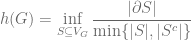
Here the notation 

Note that this is indeed like our usual isoperimetric inequalities since it’s the smallest possible ratio between size of the boundary and size of the set it encloses. In other words, this calculates the most efficient way of using small boundary to enclose areas as large as possible.
It’s of interest to find graphs with large Cheeger constant (since small Cheeger constant is easy to make: take two large graphs and connect them with a single edge).
It’s also intuitive that as the number of edges going out from each vertice become large, the Cheeger constant will become large. Hence it make sense to restrict ourselves to graphs where there are exactly 
If you play around a little bit, you will find that it’s not easy to build large k-regular graphs with Cheeger constant larger than a fixed number, say, 
Definition: A sequence of k-regular graphs 


By random methods due to Erdos, we can prove that expander families exist. However an explicit construction is much harder.
Definition: The girth of
In the case of trees, since it does not contain any non-trivial cycle, define the girth to be infinity.
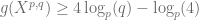
The book constructs for us, given pair 


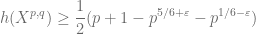
where 
Note that the bound is strictly positive and independent of 


In fact, this constructs for us an infinite family of expander families: a 
One of the crucial step in proving this is to bound the girth of the graph 

Let 


Fix odd prime


where the norm 


Define equivalence relation 


Let 

Since we know 

In elementary number theory, we know that the equation 

In each 


Let 

Check that 
We have 


Consider the Cayley graph 

Claim:
Suppose not, let 


Hence 
Since 


Since every word in 


Contradiction. Establishes the claim.
Now we reduce the group 

One can check that 
Let 

For 
Let 


Now we are ready to define our expanding family:
Since 

Theorem 1:
Let 


Let 


Also, since 
By Lemma, since 


We deduce 

Theorem 2: If
For any cycle of length 

Since 


Note that 
Hence 
Since 

If 

But we know that 

Conclude 

 .
.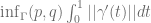
 is the collection of all differentiable curves
  connecting the two points.
 of the tangent bundle (depending continuously on the base point). We may attempt to define the metric
 is the collection of curves connecting
  for all
  . (i.e. we are only allowed to go along directions in the sub-bundle.
 -plane at all points. It’s easy to realize that now we are ‘stuck’ in the same height: any two points with different
  coordinate will have no curve connecting them (hence the distance is infinite). The resulting metric space is real number many discrete copies of
  . Of course that’s no longer homeomorphic to
  away from the original point
  going along
  real entry Heisenberg group
  (all
(all 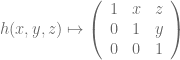
 be a left-invariant metric on
  .
. (tangent space of the identity element), the elements
 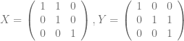 and
and  form a basis.
 of the tangent bundle generated by infinitesimal left translations by
  . Since the metric
  for each
  .
. and
and  .
.
 ,
, -direction stay the same, i.e. a bunch of horizontal lines connecting the original
  planes orthogonally.
 -direction but also adds a height
 to
to  . –since going along the
 in fact up to a constant going along such loop gives the actual distance.
 ?
? in
in  . This gives
  .
. :
:
 . (A lot shorter compare to length
  , it’s much more efficient to travel in the C-C metric.
 (meaning bounded from both inside and outside with a constant factor). Hence the volume of balls grow like
  .
.


 self-diffeomorphism of a compact subset in
  , from Whitney’s extension theorem we know exactly when does it
  is ergodic. The question is open for
  is said to be Anosov if there is a splitting of the tangent space
  that’s invariant under
  , vectors in
  are uniformly expanding and vectors in
  are uniformly contracting.
 or higher on is ergodic.
 -holder condition on the derivative.
 volume preserving diffeomorphisms are
  and a self-map
  , when can the map
  be extended to an area-preserving
  ?
? (perhaps not volume preserving) and that
  has determent
  . Whitney’s extension theorem gives a necessary and sufficient criteria for this.
 s.t.
s.t.  for all
  . When is there a
  with
with  ?
? can never have volume preserving extension.
 diffeomorphism on
  can be extended to a
  area-preserving diffeomorphism on the unit disc
  .
. , the Horseshoe map
  does not extend to a Holder continuous map preserving area on the torus.
 on the plane, one needs a rope of length at least
  .” or equivalently, given
  bounded open, we always have
 , we have
 is the volume of the unit n-ball. Note that the inequality is sharp for balls in
  be its Cayley graph, equipped with the word metric
  .
. be the cardinality of the ball of radius
  around the identity.
 , we define
  i.e. points that’s not in
  but there is an edge in the Cayley graph connecting it to some point in
  , then for any set
  ,
, .
. , so we have
  .
. , we look at how many elements of
  . (Here the idea being the size of the boundary can be lower bounded in terms of the length of the translation vector and the volume shifted outside the set. Hence we are interested in finding an element that’s not too far away from the identity but shifts a large volume of
  as
as  is:
is: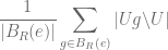
 , count how many
  outside
  .
. .
. , hence
  .
. 
 (at least as large as average).
 .
. , since
  , there must be some
  s.t.
s.t.  and
and  .
.  ,
,  .
. i.e. a union of
  .
.

 , we have
  .
.  , hence we have
 , then trancing through the argument we get bound
 . But to get that one needs to use more information of the expander than merely the volume of balls.
 then for any open set
  .
. might be strictly larger than the dimension of the manifold depending on how ‘neigatively curved’ the manifold is in large scale.
 is above average.
 ![\gamma: [0, ||g||]](https://s0.wp.com/latex.php?latex=%5Cgamma%3A+%5B0%2C+%7C%7Cg%7C%7C%5D&bg=ffffff&fg=5e5e5e&s=0&c=20201002) be a unit speed geodesic connecting
be a unit speed geodesic connecting  to
to ![\gamma([0, ||g||])](https://s0.wp.com/latex.php?latex=%5Cgamma%28%5B0%2C+%7C%7Cg%7C%7C%5D%29&bg=ffffff&fg=5e5e5e&s=0&c=20201002) , this must contain all of
, this must contain all of  since for any
  the segment
 ![\gamma([0,||g||]) \cdot u](https://s0.wp.com/latex.php?latex=%5Cgamma%28%5B0%2C%7C%7Cg%7C%7C%5D%29+%5Ccdot+u&bg=ffffff&fg=5e5e5e&s=0&c=20201002) must cross the boundary of
must cross the boundary of ![c \in [0,||g||]](https://s0.wp.com/latex.php?latex=c+%5Cin+%5B0%2C%7C%7Cg%7C%7C%5D&bg=ffffff&fg=5e5e5e&s=0&c=20201002) where
where  , hence
 .
.

 .
. 