Isoperimetric inequality on groups

February 28, 2011February 28, 2011 Conan5 Comments

Back in high school, we have all learned and loved the isoperimetric inequality: “If one wants to enclose a region of area $\pi$ on the plane, one needs a rope of length at least $2 \pi$ .” or equivalently, given $U \subseteq \mathbb{R}^2$ bounded open, we always have

$\ell(\partial U) \geq 2 \sqrt{\pi} \sqrt{\mbox{Area}(U)}$

Of course this generalizes to $\mathbb{R}^n$ :

Theorem: Given any open set $U \subseteq \mathbb{R}^n$ , we have

$\mbox{vol}_{n-1}\partial (U) \geq n\cdot \omega_n^{1/n} \mbox{vol}_n(U)^{\frac{n-1}{n}}$

Here $\omega_n$ is the volume of the unit n-ball. Note that the inequality is sharp for balls in $\mathbb{R}^n$ .

One nature question to ask should be: for which other kind of spaces do we have such an inequality. i.e. when can we lower bound the volume of the boundary by in terms of the volume of the open set? If such inequality exists, how does the lower bound depend on the volume of the set?

I recently learned to produce such bounds on groups:
Let $G$ be a discrete group, fix a set of generators and let $C_G$ be its Cayley graph, equipped with the word metric $d$ .

Let $N(R) = |B_R(e)|$ be the cardinality of the ball of radius $R$ around the identity.

For any set $U \subseteq G$ , we define $\partial U = \{g \in G \ | \ d(g, U) = 1 \}$ i.e. points that’s not in $U$ but there is an edge in the Cayley graph connecting it to some point in $U$ .

Theorem:For any group with the property that $N(R) \geq c_n R^n$ , then for any set $U \subseteq G$ with $|U| \leq \frac{1}{2}|G|$ ,

$|\partial U| \geq c_n |U|^{\frac{n-1}{n}}$ .

i.e. If the volume of balls grow (w.r.t. radius) as fast as what we have in $\mathbb{R}^n$ , then we can lower bound the size of boundary any open set in terms of its volume just like what we have in $\mathbb{R}^n$ .

Proof: We make use of the fact that right multiplications by elements of the group are isometries on Cayley graph.

Let $R = (\frac{2}{c_n}|U|)^\frac{1}{n}$ , so we have $|B_R(e)| \geq 2|U|$ .

For each element $g \in B_R(e)$ , we look at how many elements of $U$ went outside of $U$ i.e. $| Ug \backslash U|$ . (Here the idea being the size of the boundary can be lower bounded in terms of the length of the translation vector and the volume shifted outside the set. Hence we are interested in finding an element that’s not too far away from the identity but shifts a large volume of $U$ outside of $U$ .)

The average value of $|Ug \backslash U|$ as $g$ varies in the ball $B_R(e)$ is:

$\displaystyle \frac{1}{|B_R(e)|} \sum_{g\in B_R(e)} |Ug \backslash U|$

The sum part is counting the elements of $U$ that’s translated outside $U$ by $g$ then sum over all $g \in B_R(e)$ , this is same as first fixing any $u \in U$ , count how many $g$ sends $u$ outside $U$ , and sum over all $u \in U$ ( In fact this is just Fubini, where we exchange the order of two summations ). “how mant $g \in B_R(e)$ sends $u$ outside of $U$ ” is merely $|uB_R(e) \backslash U|$ .

Hence the average is

$\displaystyle \frac{1}{|B_R(e)|} \sum_{u\in U}|uB_R(e) \backslash U|$ .

But we know $|B_R(e)| \geq 2 \cdot |U|$ , hence $|uB_R(e) \backslash U|$ is at least $\frac{1}{2}|B_R(e)|$ .

Hence

$\displaystyle \frac{1}{|B_R(e)|} \sum_{u\in U}|uB_R(e) \backslash U|$

$\geq \frac{1}{|B_R(e)|} \cdot |U| \cdot \frac{1}{2} |B_R(e)| = \frac{1}{2} |U|$

Now we can pick some $g \in B_R(e)$ where $|Ug \backslash U| \geq \frac{1}{2}|U|$ (at least as large as average).

Since $g$ has norm at most $R$ , we can find a word $g_1 g_2 \cdots g_k = g, \ k \leq R$ .

For any $ug \in (Ug \backslash U)$ , since $u \in U$ and $ug \notin U$ , there must be some $1\leq i\leq k$ s.t. $u(g_1\cdots g_{i-1}) \in U$ and $u(g_1\cdots g_i) \notin U$ .

Hence $u g_1 \cdots g_i \in \partial U$ , $ug \in \partial U \cdot g_{i+1} \cdots g_k$ .

We deduce that $\displaystyle Ug \backslash U \subseteq \partial U \cup \partial U g_k \cup \cdots \cup \partial U g_2 \cdots g_k$ i.e. a union of $k$ copies of $\partial U$ .

Hence $R |\partial U| \geq k |\partial U| \geq |Ug \backslash U| \geq \frac{1}{2}|U|$

$|\partial U| \geq \frac{|U|}{2R}$

Since $|B_R(e)| \geq c_n R^n$ , we have $R \leq c_n |B_R(e)|^{\frac{1}{n}}$ . $R = (\frac{2}{c_n}|U|)^\frac{1}{n} = c_n |U|^\frac{1}{n}$ , hence we have

$|\partial U| \geq c_n |U|^\frac{n-1}{n}$

Establishes the claim.

Remark: The same argument carries through as long as we have a lower bound on the volume of balls, not necessarily polynomial. For example, on expander graphs, the volume of balls grow exponentially: $B_R(e) \geq c \cdot e^R$ , then trancing through the argument we get bound

$|\partial U| \geq c \cdot \frac{|U|}{\log{|U|}}$

Which is a very strong isoperimetric inequality. However in fact the sharp bound for expanders is $|\partial U| \geq c \cdot |U|$ . But to get that one needs to use more information of the expander than merely the volume of balls.

On the same vein, we can also prove a version on Lie groups:

Theorem:Let $G$ be a Lie group, $g$ be a left invariant metric on $G$ . If $\mbox{vol}_n(B_R) \geq c_n R^n$ then for any open set $U$ with no more than half of the volume of $G$ ,

$\mbox{vol}_{n-1}(\partial U) \geq c_n \mbox{vol}_n(U)^\frac{n-1}{n}$ .

Note that to satisfy the condition $\mbox{vol}_n(B_R) \geq c_n R^n$ , our Lie group must be at least n-dimensional since if not the condition would fail for small balls. $n$ might be strictly larger than the dimension of the manifold depending on how ‘neigatively curved’ the manifold is in large scale.

Sketch of proof: As above, take a ball twice the size of the set $U$ around the identity, say it’s $B_R(e)$ . Now we consider all left translates of the set $U$ by element in $B_R(e)$ . In average an element shifts at least half of $U$ outside of $U$ . Pick element $g$ where $\mbox{vol}(gU \backslash U)$ is above average.

Let $\gamma: [0, ||g||]$ be a unit speed geodesic connecting $e$ to $g$ . Consider the union of left translates of $\partial U$ by elements in $\gamma([0, ||g||])$ , this must contain all of $gU \backslash U$ since for any $gu \notin U$ the segment $\gamma([0,||g||]) \cdot u$ must cross the boundary of $U$ , i.e. there is $c \in [0,||g||]$ where $\gamma(c) u \in \partial U$ , hence

$g\cdot u = \gamma(||g||) \cdot u = \gamma(||g||-c)\gamma(c) u \in \gamma(||g||-c) \cdot \partial U$

But since the geodesic has derivative $1$ , the n-dimensional volume of the union of those translates is at most $\mbox{vol}_{n-1}(\partial U) \cdot ||g||$ .

We have $\mbox{vol}_{n-1}(\partial U) \cdot R \geq \mbox{vol}_n(gU \backslash U) \geq \mbox{vol}_n(U)/2$

Now since we have growth condition

$2\mbox{vol}_n(U) = \mbox{vol}_n(B_R) \geq c_n R^n$

i.e. $R \leq c_n \mbox{vol}_n(U)^\frac{1}{n}$ .

Conbine the two inequalities we obtain

$\mbox{vol}_{n-1}(\partial U) \geq c_n \mbox{vol}_n(U)^\frac{n-1}{n}$ .

Establishes the theorem.

Remark: In general, this argument produces a lower bound on the size of the boundary in terms of the volume of the set as long as:
1. There is a way to ‘continuously translate’ the set by elements in the space.
2. We have a lower bound on the growth of balls in terms of radius.

The key observation is that the translated set minus the original set is always contained in a ‘flattened cylinder’ of the boundary in direction of the translate, which then has volume controlled by the boundary size and the length of the translating element. Because of this, the constant is almost never strict as the difference (translate subtract original) can never be the whole cylinder (in case of a ball, this difference is a bit more than half of the cylinder).

On Uryson widths

February 21, 2011February 21, 2011 ConanLeave a comment

This is a note on parts of Gromov’s paper ‘width and related invariants of Riemannian manifolds’ (1988).

For a compact subset $C$ of $\mathbb{R}^n$ , we define the k-codimensional width (or simply k-width) to be the smallest possible number $w$ where there exists a k-dimensional affine subspace $P_k \subseteq \mathbb{R}^n$ s.t. all points of $C$ is no more than $w$ away from $P_k$ .

i.e.

$\displaystyle{W}_k(C) = \inf_{P_k \subseteq \mathbb{R}^n} \sup_{p\in C} \mbox{dist}(p, P_k)$
where $\mbox{dist}(p, P_k)$ is the length of the orthogonal segment from $p$ to $P_k$ .

It’s easy to see that, for any $C$ ,

$\mathcal{W}_0(C) \geq \mathcal{W}_1(C) \geq \cdots \geq \mathcal{W}_n(C) = 0$ .

At the first glance it may seems that $\mathcal{W}_0(C) = \frac{\mbox{diam}(C)}{2}$ . However it is not the case since for example the equilateral triangle of side length $1$ in $\mathbb{R}^2$ has diameter $1$ but 0-width $\frac{1}{\sqrt{3}}$ . In fact, by a theorem of Jung, this is indeed the optimum case, i.e. we have:

$\frac{1}{2}\mbox{diam}(C) \leq \mathcal{W}_0(C) \leq \sqrt{\frac{n}{2(n+1)}}\mbox{diam}(C)$

At this point one might wonder (at least I did), if we want to invent a notion that captures the ‘diameter’ after we ‘forget the longest k-dimensions’, a more direct way seem to be taking the smallest possible number $w'$ where there is an orthogonal projection of $C$ onto a $k$ dimensional subspace $P_k$ where any point $p \in P_k$ has pre-image with diameter $\leq w'$ .

i.e.

$\displaystyle \widetilde{\mathcal{W}_k}(X) = \inf_{P_k \subseteq \mathbb{R}^n} \sup_{p \in P_k} \mbox{diam}(\pi^{-1}_{P_k}(p))$

Now we easily have $\mbox{diam}(C) = \widetilde{\mathcal{W}_0}(C) \geq \widetilde{\mathcal{W}_1}(C) \geq \cdots \geq \widetilde{\mathcal{W}_n}(C) = 0$ .

However, the disadvantage of this notion is, for example, there is no reason for a semicircle arc to have 1-width 0 but a three-quarters circular arc having positive 1-width.

Since we are measuring how far is the set from being linear, taking convex hull should not make the set ‘wider’ $\widetilde{\mathcal{W}_k}$ , unlike $\widetilde{\mathcal{W}_k}$ is not invariant under taking convex hulls. Note that for convex sets we do have

$\frac{1}{2}\widetilde{\mathcal{W}_k}(C) \leq \mathcal{W}_k(C) \leq \sqrt{\frac{n-k}{2(n-k+1)}}\widetilde{\mathcal{W}_k}(C)$

$\mathcal{W}_k(C) = 0$ iff $C$ is contained in a $k$ -plane.

We now generalize this notion to general metric spaces:

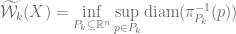
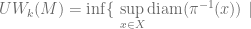
Definition: The Uryson k-width of a compact metric space $M$ is the smallest number $w$ where there exists $k$ dimensional topological space $X$ and a continuous map $\pi: M \rightarrow X$ where any point $x \in X$ has pre-image with diameter $\leq w$ .

i.e. $\displaystyle UW_k(M) = \inf \{ \ \sup_{x \in X} \mbox{diam}(\pi^{-1}(x)) \ |$

$\dim{X} = k, \pi:M \rightarrow X \ \mbox{is continuous} \}$

Note: Here dimension is the usual covering dimension for topological spaces: i.e. a topological space $X$ is $n$ dimensional if any finite cover of $X$ has a finite refinement s.t. no point of $X$ is contained in more than $n_1$ sets in the cover and $n$ is the smallest number with this property.

For compact subsets $C$ of $\mathbb{R}^n$ with induced metric, we obviously we have $UW_k(C) \leq \widetilde{\mathcal{W}_k}(C)$ since the pair $(P_k, \pi_{p_k})$ is clearly among the pairs we are minimizing over.

Speaking of topological dimensions, one of the classical results is the following:

Lebesgue’s lemma: Let $M=[0,1]^n$ be the solid n-dimensional cube, then for any topological space $X$ with $\dim(X)<n$ and any continuous map $p: M \rightarrow X$ , we have image of at least one pair of opposite $(n-1)$ -faces intersect.

Since the conclusion is purely topological, this applies equally well to rectangles. i.e. for $M = [0, L_1] \times [0, L_2] \times \cdots \times [0, L_n]$ , $L_1 \geq L_2 \geq \cdots \geq L_n$ , we have $UW_{n-1}(M) \geq L_n$ ; furthermore, $UW_k(M) \geq L_{k+1}$ for all $k$ .

(If the later statement does not hold, we write $M$ as $M_1 \times M_2$ , $M_1$ being the product of the first $(k+1)$ coordinates. Now $UW_k(M) \geq UW_k(M_1) \geq L_{k+1}$ ).

In light of the earlier post about minimax inequality, we should note that if we restrict $X$ to be a homeomorphic copy of $\mathbb{R}^k$ then the notion is the same as the minimax length of fibres. In particular as proved in the post the minimax length of the unit disc to $\mathbb{R}$ is 2.

Exercise: Check that for the unit $2$ -disk, $UW_1(D^2) = \sqrt{3}$ , i.e. the optimum is obtained by contracting the disc onto a triod.

Hence it can indeed be strictly smaller than merely taking $\mathbb{R}^k$ as the targeting space, even for simply connected sets. This gives a better measurement of ‘width’ in the sense that, for example, the $\varepsilon$ neighborhood of a tree will have $1-width$ about $2 \varepsilon$ .

Intergal geometry and the minimax inequality in a nutshell

February 7, 2011February 7, 2011 Conan1 Comment

The goal for most of the posts in this blog has been to take out some very simple parts of certain papers/subjects and “blow them up” to a point where anybody (myself included) can understand. Ideally the simple parts should give some inspirations and ideas towards the more general subject. This one is on the same vein. This one is based on parts of professor Guth’s minimax paper.

In an earlier post, we talked about the extremal length where one is able to bound the “largest possible minimum length” (i.e. the “maximum minimum length“) of a family of rectifiable curves under conformal transformation. When combined with the uniformization theorem in for surfaces, this becomes a powerful tool for understanding arbitrary Riemannian metrics (and for conformal classes of metrics in higher dimensions).

However, in ‘real life’ we often find what we really want to bound is, instead, the “minimum maximum length” of a family of curves, for example:

Question: Let $\mathbb{D} \subseteq \mathbb{R}^2$ be the unit disc. Given any family $\mathcal{F}$ of arcs with endpoints on $\partial \ \mathbb{D}$ and $\mathcal{F}$ foliates $\mathbb{D}$ , then how short can the logest arc in $\mathcal{F}$ possibly be?

In other words, let $\mathbb{F}$ be the collection of all possible such foliations $\mathcal{F}$ as above, what is

$\displaystyle \inf_{\mathcal{F} \in \mathbb{F}} \ \sup_{A \in \mathcal{F}} \ \ell(A)$ ?

After playing around a little bit with those foliations, we should expect one of the fibres to be at least as long as the diameter ( i.e. no foliation has smaller maximum length leaf than foliating by straight lines ). Hence we should have

$\displaystyle \inf_{\mathcal{F} \in \mathbb{F}} \ \sup_{A \in \mathcal{F}} \ \ell(A) = 2$ .

This is indeed easy to prove:

Proof: Consider the map $f: S^1 \rightarrow S^1$ where $S^1 = \partial \ \mathbb{D}$ , $f$ switches the end-points of each arc in $\mathcal{F}$ . It is easy to check that $f$ is a continuous, orientation reversing homeomorphism of the circle (conjugate to a reflection). Let $p, q$ be its fixed points, $L_1, L_2$ be the two arcs in $S^1$ connecting $p$ to $q$ .

Let

$g: z \mapsto -z$

be the antipodal map on $S^1$ .

Suppose $p \neq g(q)$ then one of $L_1, L_2$ is longer than $\pi$ , say it’s $L_1$ .

Then we have

$f \circ g (L_1) \subseteq L_1$ .

Hence $f \circ g$ has a fixed point $m$ in $L_1$ , i.e. $f(m) = -m$ .

There is a fibre $A$ in $\mathcal{F}$ with endpoints $m, -m$ , the fibre must have length

$\ell(A) \geq d(-m,m) = 2$ .

The remaining case is trivial: if $p = g(q)$ then both $L_1$ and $L_2$ gets mapped into themselves orientation-reversingly, hence fixed points still exists.

Establishes the claim.

Instead of the disc, we may look at circles that sweep out the sphere (hence to avoid the end-point complications):

Theorem: Any one-parameter family of circles that foliates $S^2$ (except two points) must have the largest circle being longer than the equator.

This is merely applying the same argument, i.e. one of the circles needs to contain a pair of antipodal points hence must be longer than the equator.

In order for easier generalization to higher dimensions, with slight modifications, this can be formulated as:

Theorem: For any $f: T^2 \rightarrow S^2$ having non-zero degree, there is $\theta \in S^1$ where $\ell(f(S^1 \times \{ \theta \})$ is larger than the equator.

Hence in higher dimensions we can try to prove the same statement for largest image of a lever $k$ -sphere under $f: S^k \times S^{n-k} \rightarrow S^n$ . However before we do that I would like to highlight some intergal geometry machineries that are new to me but seemingly constantly used in proving those kinds of estimates. We shall get some idea of the method by showing:

Theorem: Let $\mathbb{R}P^n$ be equipped with the round metric. $p^k \subseteq \mathbb{R}P^n$ be a ‘flat’ $k$ -dimensional plane. Then any $k$ -chain $z^k \subseteq \mathbb{R}P^n$ in the same $k$ dimensional homology class as $p^k$ must have volume at least as large as $p^k$ .

Proof: Let $Gr(\mathbb{R}P^n, n-k)$ be the set of all $(n-k)$ -planes in $\mathbb{R}P^n$ (i.e. the Grassmannian).

There is a standard way to associate a measure $\mu$ on $Gr(\mathbb{R}P^n, n-k)$ :

Let $\lambda$ be the Haar measure on $SO(n+1)$ , fix some $Q \in Gr(\mathbb{R}P^n, n-k)$ .

Since $SO(n+1)$ acts on $\mathbb{R}P^n$ , for open set $S \subseteq Gr(\mathbb{R}P^n, n-k)$ , we set

$\mu(S) = \lambda( \{ T \in SO(n+1) \ | \ T(Q) \in S \})$ .

–The measure of a collection of planes is the measure of linear transformations that takes the given plane to an element of the set.

Now we are able to integrate over all $(n-k)$ -planes!

For almost all $Q \in Gr(\mathbb{R}P^n, n-k)$ , since $P$ is $k$ -plane, we have $| Q \cap P | = 1$ . ( not $1$ only when they are ‘parallel’ )

Since $[z] = [p]$ in $H_k(\mathbb{R}P^n, \mathbb{Z}_2)$ , for almost all $Q$ , $z$ intersects $Q$ at least as much as $P$ does. We conclude that for almost all $Q, \ | z \cap Q | \geq 1$ .

Fact: There exists constant $C$ such that for any $k$ -chain $\Sigma^k \in \mathbb{R}P^N$ ,

$\mbox{Vol}_k(\Sigma^k) = \mathbb{E}(|\Sigma \cap Q |)$ .

The fact is obtained by diving the chain into fine cubes, observe that both volume and expectation are additive and translation invariant. Therefore we only need to show this for infinitesimal cubes (or balls) near $0$ . We won’t work out the details here.

Hence in our case, since for almost all $Q$ we have $| z \cap Q | \geq 1$ , the expectation $\mathbb{E}(|z \cap Q |) \geq 1$ .

We therefore deduce

$\mbox{Vol}_k(z) = \mathbb{E}(|z \cap Q |) \geq 1$ .

Establishes the theorem.

Remark: I found this intergal geometry method used here being very handy: in the old days I always try to give lower bounds on volume of stuff by intersecting it with planes and then pretend the ‘stuff’ were orthogonal to the plane, which is the worst case in terms of having small volume. An example of such bound can be found in the knot distorsion post where in order to lower bound the length we look at its intersection number with a family of parallel planes and then integrate the intersection.

This is like looking from one particular direction and record how many times did a curve go through each height, of course one would never get the exact length if we know the curve already. What if we are allowed to look from all directions?

I always wondered if we know the intersection number with not only a set of parallel planes but planes in all directions, then are there anything we can do to better bound the volume? Here I found the perfect answer to my question: by integrating over the Grassmannian, we are able to get the exact volume from how much it intersect each plane!

We get some systolic estimates as direct corollaries of the above theorem, for example:

Corollary: $\mbox{Sys}_1(\mathbb{R}P^2) = \sqrt{\pi/2}$ where $\mathbb{R}P^2$ carries the round metric with total volume $1$ .

Back to our minimax problems, we state the higher dimensional version:

Wish: For any $C^1$ map $f: S^k \times S^{n-k} \rightarrow S^n$ where $S^n$ carries the standard round metric, there exists some $\theta \in S^{n-k}$ with

$\mbox{Vol}_k(f(S^k\times \{\theta\})) \geq \mbox{Vol}_k(E^k)$

where $E^k \subseteq S^n$ is the $k$ -dimensional equator.

But what we have is that there is a (small) positive constant $c(n,k)$ s.t. $\mbox{deg}(f) \neq 0$ implies

$\displaystyle \sup_{\theta \in S^{n-k}} \mbox{Vol}_k(f(S^k \times \{\theta\})) \geq c(n,k) \mbox{Vol}_k(E^k)$

(shown by an inductive application of the isomperimetric inequality on $S^N$ , which is obtained from applying intergal geometry methods)

On length and volume

November 29, 2010December 1, 2010 Conan2 Comments

About a year ago, I came up with an simple argument for the following simple theorem that appeared in a paper of professor Guth’s:

Theorem: If $U$ is an open set in the plane with area $1$ , then there is a continuous function $f$ from $U$ to the reals, so that each level set of $f$ has length at most $10$ .

Recently a question of somewhat similar spirit came up in a talk of his:

Question: Let $\langle \mathbb{T}^2, g \rangle$ be a Riemannian metric on the torus with total volume $1$ , does there always exist a function $f: \mathbb{T}^2 \rightarrow \mathbb{R}$ s.t. each level set of $f$ has length at most $10$ ?

I have some rough thoughts about how might a similar argument on the torus look like, hence I guess it would be a good idea to review and (somewhat carefully) write down the original argument. Since our final goal now is to see how things work on a torus (or other manifolds), here I would only present the less tedious version where $U$ is bounded and all boundary components of $U$ are smooth Jordan curves. Here it goes:

Proof: Note that if a projection of $U$ in any direction has length (one-dimensional measure) $\leq 10$ , then by taking $f$ to be the projection in the orthogonal direction, all level sets are straight with length $\leq 10$ (see image below).

Hence we can assume any $1$ -dimensional projection of $U$ has length $\geq 10$ . A typically bad set would ‘span’ a long range in all directions with small area, it can contain ‘holes’ and being not connected:

Project $U$ onto $x$ and $y$ -axis, by translating $U$ , we assume $\inf \pi_x(U) = \inf \pi_y(U) = 0$ . Look at the measure $1$ set $S$ in the middle of $\pi_y(U)$ (i.e. a measure 1 set $[a,b] \cap \pi_y(U)$ with the property $m_1(\pi_y(U) \cap [0,a]) = m_1(\pi_y(U) \cap [b, \infty]$ )

By Fubini, since the volume $\pi_y^{-1}(S)$ is at most $1$ , there must be a point $p\in S$ with $m_1(\pi_y^{-1}(p))\leq 1$ :

Since the boundary of $U$ is smooth, we may find a very small neighborhood $B_\delta(p) \subseteq \mathbb{R}$ where for each $q \in B_\delta(p), m_1(\pi_y^{-1}(q) \leq 1+\epsilon$ . (we will call this pink region a ‘neck’ of the set for it has small width and is roughly in the middle)

Now we define a $\varphi_1: U \rightarrow \mathbb{R}^2$ that straches the neck to fit in a long thin tube (note that in general $\pi_y(U)$ may not be connected, but everything is still well-defined and the argument does go through.) and then bend the neck to make the top chunk vertically disjoint from the bottom chunk.

We can take $\varphi$ so that $\varphi^{-1}$ sends the vertical foliation of $\varphi(U)$ to the following foliation in $U$ (note that here we drew the neck wider for easier viewing, in fact the horizontal lines are VERY dense in the neck).

If the $y$ -projection of the top or bottom chunk is larger than $2$ , we repeat the above process t the chunks. i.e. Finding a neck in the middle measure $1$ set in the chunk, starch the neck and shift the top chunk, this process is guaranteed to terminate in at most $m_1(\pi_y(U))$ steps. The final $\varphi$ sends $U$ to something like:

Where each chunk has $y$ -width $L$ between $1$ and $2$ .

Define $f = \pi_x \circ \phi$ .

Claim: For any $c \in \mathbb{R}, m_1(f^{-1}(c)) \leq 5$ .

The vertical line $x=c$ intersects $\varphi(U)$ in at most one chunk and two necks, taking $\varphi^{-1}$ of the intersection, this is a PL curve $C$ with one vertical segment and two horizontal segment in $U$ :

The total length of $f^{-1}(c) = C \cap U$ is less than $2+2\delta$ (length of $U$ on the vertical segment) $+ 2 \times (1+\epsilon)$ (length of $U$ on each horizontal segment). Pick $\epsilon, \delta$ both less than $1/4$ , we conclude $m_1(f^{-1}(c)) < 5$ .

Establishes the theorem.

Remark:More generally,any open set of volume $V$ has such function with fibers having length $\leq 5 \sqrt{V}$ . T he argument generalizes by looking at the middle set length $\sqrt{V}$ set of each chunk.

Moving to the torus

Now let’s look at the problem on $\langle \mathbb{T}^2, g \rangle$ , by the uniformization theorem we have a flat torus $T^2 = \mathbb{R}^2/\Gamma$ where $\Gamma$ is a lattice, $\mbox{vol}(T^2) = 1$ and a function $h: T^2 \rightarrow \mathbb{R}^{+}$ s.t. $\langle T^2, h g_0 \rangle$ is isometric to $\langle \mathbb{T}^2, g \rangle$ . $g_0$ is the flat metric. Hence we only need to find a map on $T^2$ with short fibers.

Note that

$\int_{T^2} h^2 d V_{g_0} = 1$

and the length of the curve $\gamma$ from $p$ to $q$ in $\langle T^2, h \dot{g_0} \rangle$ is

$\int_I h |\gamma'(t)| dt$ .

Consider $T^2$ as the parallelogram given by $\Gamma$ with sides identified. w.l.o.g. assume one side is parallel to the $x$ -axis. Let $L$ be a linear transformation preserving the horizontal foliation and sends the parallelogram to a rectangle.

Let $F$ be a piece-wise isometry that “folds” the rectangle:

(note that $F$ is four-to-one except for on the edges and the two medians)
Since all corresponding edges are identified, $lates F$ is continuous not only on the rectangle but on the rectangular torus.

Now we consider $F \circ L$ , pre-image of typical horizontal and vertical lines in the small rectangle are union of two parallel loops:

Note that vertical loops might be very long in the flat $T^2$ due to the shear while the horizontal is always the width.

(to be continued)

Systoles and the generalized Geroch conjecture

October 25, 2010November 1, 2011 Conan3 Comments

Almost a year ago, I said here that I would write a sequence of posts on some simple facts and observations related to the systolic inequality but got distracted and didn’t manage to do much of that…

I was reminded last week as I heard professor Guth’s talk on systoles for the 4th time (Yes, the same talk! –in Toronto, Northwestern, India and here at the IAS). It’s interesting that I’m often thinking about different things each time I hear the same talk. This one is about the generalized Geroch conjecture.

Geroch conjecture: $\mathbb{T}^n$ (the $n$ -torus) does not admit a metric of positive scalar curvature.

The conjecture is proved by Schoen and Yau (1979).

Now, scalar curvature can be seen as a limit of volume of balls:

Definition: The scalar curvature of $M$ at $p$ is

$\displaystyle \mbox{Sc}(p) = c_n \lim_{r\rightarrow 0} \frac{\mbox{Vol}_E (B(\bar{0},r)) - \mbox{Vol}_g(B(p,r))}{r^{n+2}}$

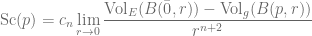
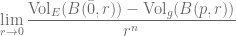
where $\mbox{Vol}_E$ is the Euclidian volume and $c_n$ is a positive constant only depending on the dimension $n$ .

Note that since our manifold does not have any cone points,

$\displaystyle \lim_{r\rightarrow 0} \frac{\mbox{Vol}_E (B(\bar{0},r)) - \mbox{Vol}_g(B(p,r))}{r^n}$

must vanish. Further more, the Riemannian structure on $M$ forces the $r^{n+1}$ term to vanish.

Since for this context we only care about is whether the scalar curvature is larger or smaller than $0$ , we can be even more simple-minded: $M$ has positive scalar curvature at $p$ all small enough balls around $p$ has smaller volume than their Euclidean cousins (with a difference of order propositional to $r^{n+2}$ ). In light of this definition, we have:

Restatement of the Geroch conjecture: For all $g$ on $\mathbb{T}^n$ , there exists some point $p$ s.t. $\mbox{Sc}(p) \leq 0$ .

This is to say, small enough balls around some point $p$ are not small enough for it to have positive scalar curvature. What if instead we look at balls of a fixed radius instead of those infinitesimal balls? This naturally leads to

Generalized Geroch conjecture: For any $(\mathbb{T}^n, g)$ , for all $r$ , there exists $p$ s.t. $\mbox{Vol}_g(B(p, r)) \geq \mbox{Vol}_E(B(\bar{0}, r))$ .

(For those $r$ larger than the injectivity radius, we lift $M$ to its universal cover so that all homotopically non-trival loops are ‘unfolded’)

Let’s take a look at the $2$ -torus to get a feel of the conjecture:

The flat torus, of course, has $0$ $r$ -scalar curvature at all points.

For the regular rotational torus, we take the ball around the saddle point of the gradient flow, the ball look like a saddle, as shown below.

To see that this has area larger than the analogous Euclidean ball, we can cut it along radial rays into thin triangles, each triangle can be ‘almost flattened’ to a Euclidean triangle, but we have a more triangles than in the Euclidean case.

What if we try to make the surface spherical for most of the area and having those negative scalar curvature points taking up a very small potion. One of my first attempts would be to connect a few spheres with cylinders:

We have a few parameters here: the number of balls $n$ , the width of the connecting cylinders $w$ , the length of the connecting cylinders $l$ and the radius of each sphere $R$ .

If cylinders are too long (longer than $2r$ ), then we can just take the ball in the middle of the cylinder, the volume when lifted to universal cover would be equal to Euclidean.

If the width of cylinders are much smaller than $r$ , then the ball around a point in the gluing line would have volume almost a full spherical ball plus a half Euclidean ball, which would obviously be larger than a full Euclidean ball.

Hence the more interesting case is to have very short, wide tubes and as a consequence, have many balls forming a loop. In this case, the ‘worst’ ball would be centered at the middle of the tube, it intersects the two spheres connected by the tube in something a bit larger than a spherical half-ball.

I haven’t figured out an estimate yet. i.e. can the advantage taken from the fact that spherical ball are smaller than Euclidean balls cancel out the ‘a bit larger than half’? I think that would be interesting to work out.

Finally, let’s say what does this has to do with systoles:

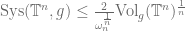
Theorem: Generalized Geroch conjecture $\Rightarrow$ $\mbox{Sys}(\mathbb{T}^n, g) \leq \frac{2}{\omega_n^{\frac{1}{n}}} \mbox{Vol}_g(\mathbb{T}^n)^{\frac{1}{n}}$ (which is the systolic inequality with a constant better than what we have so far)

Proof: Suppose not,

$\mbox{Sys}(\mathbb{T}^n, g) > 2 (\frac{\mbox{Vol}_g(\mathbb{T}^n)}{\omega_n})^{\frac{1}{n}}$

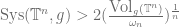
Let $r = (\frac{\mbox{Vol}_g(\mathbb{T}^n)}{\omega_n})^{\frac{1}{n}}$ , by the generalized Geroch conjecture we have some $B(p, r)$ larger than the Euclidean ball. i.e.

$\mbox{Vol}_g(B(p, r))>\omega_n r^n = \omega_n \frac{\mbox{Vol}_g(\mathbb{T}^n)}{\omega_n} = \mbox{Vol}_g(\mathbb{T}^n)$

Since the systole is at least $2r$ , hence $B(p, r)$ cannot contain any homotopically non-trival loop i.e. it does not “warp around” and get unfolded when passing to the universal cover. Hence volume of a ball with radius $r$ cannot be larger than the volume of the whole manifold. Contradiction

Area777

Chasing dreams from mathematics to the real world

Tag: Larry Guth

Isoperimetric inequality on groups

On Uryson widths

Intergal geometry and the minimax inequality in a nutshell

On length and volume

Systoles and the generalized Geroch conjecture

Share this:

Share this:

Share this:

Share this:

Share this: