Well, some people might be wondering why I haven’t updated my blog since two weeks ago…Here’s the answer: I have been preparing for this generals exam — perhaps the last exam in my life.
For those who don’t know the game rules: The exam consists of 3 professors (proposed by the kid taking the exam, approved by the department), 5 topics (real, complex, algebra + 2 specialized topics chosen by the student). One of the committee member acts as the chair of the exam.
The exam consists of the three committee members sitting in the chair’s office, the student stands in front of the board. The professors ask questions ranging in those 5 topics for however long they want, the kid is in charge of explaining them on the board.
I was tortured for 4.5 hours (I guess it sets a new record?)
I have perhaps missed some questions in my recollection (it’s hard to remember all 4.5 hours of questions).
Conan Wu’s generals
Commitee: David Gabai (Chair), Larry Guth, John Mather
Topics: Metric Geometry, Dynamical Systems
Real analysis:
Mather: Construct a first category but full measure set.
(I gave the intersection of decreasing balls around the rationals)
Guth: 
(Decreasing faster than 
Mather: Does integration by parts work for Lipschitz functions?
(Lip imply absolutely continuous then Lebesgue’s differentiation theorem)
Mather: If one only has bounded variation, what can we say?
(
Mather: If 
(Prove it’s rapidly decreasing)
Mather: Given a smooth 


(A necessary condition is the integral of 
I had to expand everything in Fourier coefficients, show that if 


Gabai: Write down a smooth function from 
(I wrote 

Gabai: Can you find a such function with the level curves form a different foliation from this one?
(I think he meant that two foliations are different if there is no homeo on 
After playing around with it for a while, I came up with an example where the level sets form a Reeb foliation, and that’s not same as the lines!)
We moved on to complex.
Complex analysis:
Guth: Given a holomorphic 


(with a bunch of hints/suggestions, I finally got 
Guth: State maximal modulus principal.
Gabai: Define the Mobius group and how does it act on 
Gabai: What do the Mobius group preserve?
(Poincare metric)
Mather: Write down the Poincare metric, what’s the distance from 

(I don’t remember the exact distance form, so I tried to guess the denominator being 

Gabai: Suppose I have a finite subgroup with the group of Mobius transformations acting on 
(I sketched an argument based on each element having finite order must have a unique fixed point in the interior of
I think that’s pretty much all for the complex.
Algebra:
Gabai: State Eisenstein’s criteria
(I stated it with rings and prime ideals, which leaded to a small discussion about for which rings it work)
Gabai: State Sylow’s theorem
(It’s strange that after stating Sylow, he didn’t ask me do anything such as classify finite groups of order xx)
Gabai: What’s a Galois extension? State the fundamental theorem of Galois theory.
(Again, no computing Galois group…)
Gabai: Given a finite abelian group, if it has at most 
(classification of abelian groups, induction, each Sylow is cyclic)
Gabai: Prove multiplicative group of a finite field is cyclic.
(It’s embarrassing that I was actually stuck on this for a little bit before being reminded of using the previous question)
Gabai: What’s 
(I said linear automorphisms on the torus. I thought it can only be 

Gabai: What’s 
(
Gabai: For any closed orientable 

(Poincare duality + universal coefficient)
We then moved on to special topics:
Metric Geometry:
Guth: What’s the systolic inequality?
(the term ‘aspherical’ comes up)
Gabai: What’s aspherical? What if the manifold is unbounded?
(I guessed it still works if the manifold is unbounded, Guth ‘seem to’ agree)
Guth: Sketch a proof of the systolic inequality for the n-torus.
(I sketched Gromov’s proof via filling radius)
Guth: Give an isoperimetric inequality for filling loops in the 3-manifold 

(My guess is for any 2-chain we should have

then I tried to prove that using some kind of random cone and grid-pushing argument, but soon realized the method only prove

Guth: Given two loops of length 

(it can be as large as 
Dynamical Systems:
Mather: Define Anosov diffeomorphisms.
Mather: Prove the definition is independent of the metric.
(Then he asked what properties does Anosov have, I should have said stable/unstable manifolds, and ergodic if it’s more than 
Mather: Prove structural stability of Anosov diffeomorphisms.
(This is quite long, so I proposed to prove Anosov that’s Lipschitz close to the linear one in 
Mather: Define Anosov flow, what can you say about geodesic flow for negatively curved manifold?
(They are Anosov, I tried to draw a picture to showing the stable and unstable and finished with some help)
Mather: Define rotation number, what can you say if rotation numbers are irrational?
(They are semi-conjugate to a rotation with a map that perhaps collapse some intervals to points.)
Mather: When are they actually conjugate to the irrational rotation?
(I said when 

I do not know why, but at this point he wanted me to talk about the fixed point problem of non-separating plane continua (which I once mentioned in his class).
After that they decided to set me free~ So I wandered in the hallway for a few minutes and the three of them came out to shake my hand.
 .
. is defined as
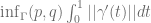
 is the collection of all differentiable curves
  connecting the two points.
 of the tangent bundle (depending continuously on the base point). We may attempt to define the metric
 is the collection of curves connecting
  for all
  . (i.e. we are only allowed to go along directions in the sub-bundle.
 -plane at all points. It’s easy to realize that now we are ‘stuck’ in the same height: any two points with different
  coordinate will have no curve connecting them (hence the distance is infinite). The resulting metric space is real number many discrete copies of
  away from the original point
  can be connected to
  going along
  real entry Heisenberg group
  (all
(all 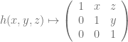
 .
. (tangent space of the identity element), the elements
 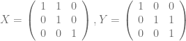 and
and  form a basis.
 of the tangent bundle generated by infinitesimal left translations by
  . Since the metric
  for each
  .
. and
and  .
.
 ,
, -direction stay the same, i.e. a bunch of horizontal lines connecting the original
  planes orthogonally.
 -direction but also adds a height
 to
to  . –since going along the
 in fact up to a constant going along such loop gives the actual distance.
 ?
? in
in  . This gives
  .
. :
:
 . (A lot shorter compare to length
  for going
  , it’s much more efficient to travel in the C-C metric.
 is roughly an rectangle with dimension
  (meaning bounded from both inside and outside with a constant factor). Hence the volume of balls grow like
  .
.
 on the plane, one needs a rope of length at least
  .” or equivalently, given
  bounded open, we always have
 , we have
 is the volume of the unit n-ball. Note that the inequality is sharp for balls in
  be a discrete group, fix a set of generators and let
  be its Cayley graph, equipped with the word metric
  .
. be the cardinality of the ball of radius
  around the identity.
 , we define
  i.e. points that’s not in
  but there is an edge in the Cayley graph connecting it to some point in
  , then for any set
  ,
, .
. , so we have
  .
. , we look at how many elements of
  . (Here the idea being the size of the boundary can be lower bounded in terms of the length of the translation vector and the volume shifted outside the set. Hence we are interested in finding an element that’s not too far away from the identity but shifts a large volume of
  as
as  is:
is: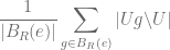
 , count how many
  outside
  .
. .
. , hence
  .
. 
 (at least as large as average).
 .
. , since
  , there must be some
  s.t.
s.t.  and
and  .
.  ,
,  .
. i.e. a union of
  copies of
  .
.

 , we have
  .
.  , hence we have
 , then trancing through the argument we get bound
 . But to get that one needs to use more information of the expander than merely the volume of balls.
 then for any open set
  .
. is above average.
 ![\gamma: [0, ||g||]](https://s0.wp.com/latex.php?latex=%5Cgamma%3A+%5B0%2C+%7C%7Cg%7C%7C%5D&bg=ffffff&fg=5e5e5e&s=0&c=20201002) be a unit speed geodesic connecting
be a unit speed geodesic connecting  to
to ![\gamma([0, ||g||])](https://s0.wp.com/latex.php?latex=%5Cgamma%28%5B0%2C+%7C%7Cg%7C%7C%5D%29&bg=ffffff&fg=5e5e5e&s=0&c=20201002) , this must contain all of
, this must contain all of  since for any
  the segment
 ![\gamma([0,||g||]) \cdot u](https://s0.wp.com/latex.php?latex=%5Cgamma%28%5B0%2C%7C%7Cg%7C%7C%5D%29+%5Ccdot+u&bg=ffffff&fg=5e5e5e&s=0&c=20201002) must cross the boundary of
must cross the boundary of ![c \in [0,||g||]](https://s0.wp.com/latex.php?latex=c+%5Cin+%5B0%2C%7C%7Cg%7C%7C%5D&bg=ffffff&fg=5e5e5e&s=0&c=20201002) where
where  , hence
 .
.

 .
.  of
of  where there exists a k-dimensional affine subspace
  s.t. all points of
  .
.
 is the length of the orthogonal segment from
  .
.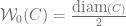 . However it is not the case since for example the equilateral triangle of side length
  . In fact, by a theorem of
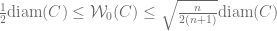
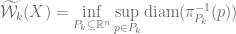
 where there is an orthogonal projection of
  has pre-image with diameter
  .
.
 .
. , unlike
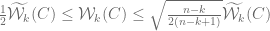
 iff
iff  where any point
  has pre-image with diameter
  .
.

 sets in the cover and
  since the pair
  is clearly among the pairs we are minimizing over.
![M=[0,1]^n](https://s0.wp.com/latex.php?latex=M%3D%5B0%2C1%5D%5En&bg=ffffff&fg=5e5e5e&s=0&c=20201002) be the solid n-dimensional cube, then for any topological space
be the solid n-dimensional cube, then for any topological space  and any continuous map
  , we have image of at least one pair of opposite
  -faces intersect.
![M = [0, L_1] \times [0, L_2] \times \cdots \times [0, L_n]](https://s0.wp.com/latex.php?latex=M+%3D+%5B0%2C+L_1%5D+%5Ctimes+%5B0%2C+L_2%5D+%5Ctimes+%5Ccdots+%5Ctimes+%5B0%2C+L_n%5D&bg=ffffff&fg=5e5e5e&s=0&c=20201002) ,
,  , we have
  ; furthermore,
  for all
  ,
,  being the product of the first
  coordinates. Now
  ).
). then the notion is the same as the minimax length of fibres. In particular as proved in the post the minimax length of the unit disc to
  is 2.
is 2. -disk,
  , i.e. the optimum is obtained by contracting the disc onto a triod.
 neighborhood of a tree will have
  about
about  .
. be the unit disc. Given any family
  of arcs with endpoints on
  and
and  be the collection of all possible such foliations
  ?
? .
. where
where  ,
,  connecting
  .
.
 then one of
  .
. .
. has a fixed point
  in
in  .
. in
in  , the fibre must have length
 .
. then both
  gets mapped into themselves orientation-reversingly, hence fixed points still exists.
 having non-zero degree, there is
  where
where  is larger than the equator.
 . However before we do that I would like to highlight some intergal geometry machineries that are new to me but seemingly constantly used in proving those kinds of estimates. We shall get some idea of the method by showing:
 be equipped with the round metric.
  be a ‘flat’
  in the same
  must have volume at least as large as
  be the set of all
  -planes in
  on
on  be the Haar measure on
  , fix some
  .
. , we set
 .
. is
is  . ( not
 ![[z] = [p]](https://s0.wp.com/latex.php?latex=%5Bz%5D+%3D+%5Bp%5D&bg=ffffff&fg=5e5e5e&s=0&c=20201002) in
in  , for almost all
  ,
,  .
. ,
, .
. , the expectation
  .
. .
. where
where  carries the round metric with total volume
  carries the standard round metric, there exists some
  with
with
 is the
  s.t.
s.t.  implies
 , which is obtained from applying intergal geometry methods)